4. Unsupervised Learning: Density Estimation
Density estimation is the act of estimating a continuous density field from a discretely sampled set of points drawn from that density field. Some examples of density estimation can be found in book_fig_chapter6
4.1. Bayesian Blocks: Histograms the Right Way
One of the simplest density estimation techniques is the histogram, usually done in one dimension. Though seemingly simple, the effective use histograms can be surprisingly subtle. Consider the following two panels:
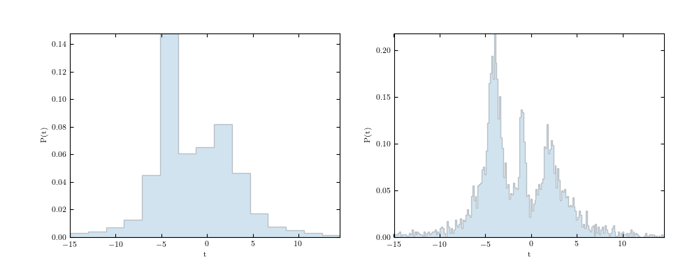
Though it doesn’t look like it, these two histograms show the exact same dataset (if you find that hard to believe, see the source code that generated the figure by clicking on the image). The difference between the two is the bin size: this illustrates the importance of choosing the correct bin size when visualizing a dataset. In practice, scientists often address this through trial and error: plot the data a few times until it looks “right”. But what does it mean for histogram data to look right?
There have been a number of solutions proposed to address this problem. They range from simple rules-of-thumb to more sophisticated procedures based on Bayesian analysis of the data. Some of the simpler examples used in the literature are Scott’s Rule 1 and the Freedman-Diaconis Rule 2. Both are based on assumptions about the form of the underlying data distribution. A slightly more rigorous approach is Knuth’s rule 3, which is based on optimization of a Bayesian fitness function across fixed-width bins. A further generalization of this approach is that of Bayesian Blocks, which optimizes a fitness function across an arbitrary configuration of bins, which need not be of equal width 4. For an approachable introduction to the principles behind Bayesian Blocs, see this blog post.
The function astroML.plotting.hist() implements all four of these
approaches to histogram binning in a natural way. It can be used as follows:
import numpy as np
from astroML.plotting import hist
x = np.random.normal(size=1000)
hist(x, bins='blocks')
The syntax is identical to the hist() function in matplotlib
(including all additional keyword arguments) with the sole exception that
the bins argument also accepts a string, which can be one of
'blocks', 'knuth', 'scott', or 'freedman'.
Using one of these causes the histogram binning to be chosen using the
rules or procedures outlined above. The results on our data using Knuth’s
rule and Bayesian Blocks are shown below:
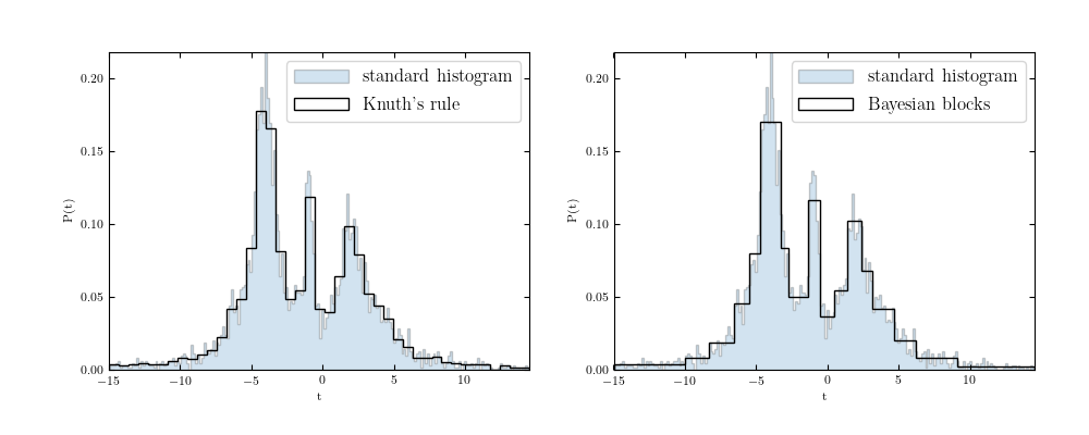
The Knuth bins on the left do a good job of representing the underlying structure of the data. The Bayesian Blocks on the right capture most of the same features, but notice that the lack of density variation in the outer regions is recognized by the Bayesian blocks procedure, which settles on very wide bins in these regions.
The utility of the Bayesian blocks approach goes beyond simple data representation, however: the bins can be shown to be optimal in a quantitative sense, meaning that the histogram becomes a powerful statistical measure. For example, if the data is consistent with a uniform distribution, the Bayesian blocks representation will reflect this by choosing a single wide bin.
4.1.1. References
- 1
Scott, D. (1979). On optimal and data-based histograms http://biomet.oxfordjournals.org/content/66/3/605
- 2
Freedman, D. & Diaconis, P. (1981). On the histogram as a density estimator: L2 theory http://www.springerlink.com/content/mp364022824748n3/
- 3
Knuth, K. H. (2006). Optimal Data-Based Binning for Histograms http://adsabs.harvard.edu/abs/2006physics…5197K
- 4
Scargle, J. et al. (2012) Studies in Astronomical Time Series Analysis. VI. Bayesian Block Representations http://adsabs.harvard.edu/abs/2012arXiv1207.5578S
4.2. Extreme Deconvolution
Extreme deconvolution is a powerful extension of Gaussian Mixture Models which
takes into account data errors and projections 5.
It is implemented in astroML
using the object astroML.density_estimation.XDGMM.
See book_fig_chapter6_fig_XD_example or
book_fig_chapter6_fig_stellar_XD
for some examples of this approach.
4.2.1. References
- 5
Bovy, J. et al. (2009). Extreme deconvolution: Inferring complete distribution functions from noisy, heterogeneous and incomplete observations. http://arxiv.org/abs/0905.2979
4.3. Kernel Density Estimation
Kernel Density estimation (KDE) is a non-parametric density estimation
technique which can be very powerful. The estimator has been deprecated and
removed from astroML in favor of sklearn.neighbors.KernelDensity,
which was added in Scikit-learn version 0.14. See
book_fig_chapter6_fig_great_wall ,
book_fig_chapter6_fig_great_wall_KDE or
book_fig_chapter6_fig_density_estimation for examples of how kernel
density estimation is used.
4.4. Nearest Neighbors Density Estimation
Nearest Neighbors Density estimation can be a fast alternative to KDE, and is
similar to KDE with a hard-edged kernel.
It is implemented in astroML using the object
astroML.density_estimation.KNeighborsDensity.
See book_fig_chapter6_fig_great_wall or
book_fig_chapter6_fig_density_estimation for examples of how it
is used.