SDSS Moving Object Catalog

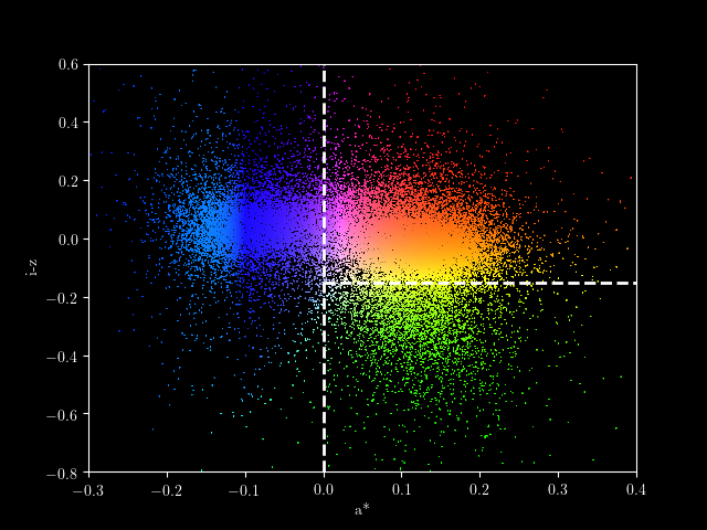
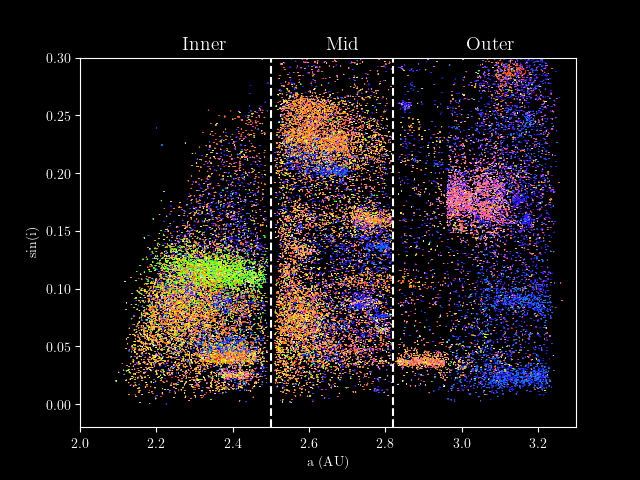
This plot demonstrates how to fetch data from the SDSS Moving object catalog, and plot using a multicolor plot similar to that used in figures 3-4 of 1

References

1

Parker et al. 2008 http://adsabs.harvard.edu/abs/2008Icar..198..138P

Code output:

Python source code:

# Author: Jake VanderPlas <vanderplas@astro.washington.edu>
# License: BSD
#   The figure is an example from astroML: see http://astroML.github.com
import numpy as np
import matplotlib
from matplotlib import pyplot as plt
from astroML.datasets import fetch_moving_objects
from astroML.plotting.tools import devectorize_axes


def black_bg_subplot(*args, **kwargs):
    """Create a subplot with black background"""

    if int(matplotlib.__version__[0]) >= 2:
        kwargs['facecolor'] = 'k'
    else:
        kwargs['axisbg'] = 'k'

    ax = plt.subplot(*args, **kwargs)

    # set ticks and labels to white
    for spine in ax.spines.values():
        spine.set_color('w')

    for tick in ax.xaxis.get_major_ticks() + ax.yaxis.get_major_ticks():
        for child in tick.get_children():
            child.set_color('w')

    return ax


def compute_color(mag_a, mag_i, mag_z, a_crit=-0.1):
    """
    Compute the scatter-plot color using code adapted from
    TCL source used in Parker 2008.
    """
    # define the base color scalings
    R = np.ones_like(mag_i)
    G = 0.5 * 10 ** (-2 * (mag_i - mag_z - 0.01))
    B = 1.5 * 10 ** (-8 * (mag_a + 0.0))

    # enhance green beyond the a_crit cutoff
    i = np.where(mag_a < a_crit)
    G[i] += 10000 * (10 ** (-0.01 * (mag_a[i] - a_crit)) - 1)

    # normalize color of each point to its maximum component
    RGB = np.vstack([R, G, B])
    RGB /= RGB.max(0)

    # return an array of RGB colors, which is shape (n_points, 3)
    return RGB.T


#------------------------------------------------------------
# Fetch data and extract the desired quantities
data = fetch_moving_objects(Parker2008_cuts=True)
mag_a = data['mag_a']
mag_i = data['mag_i']
mag_z = data['mag_z']
a = data['aprime']
sini = data['sin_iprime']

# dither: magnitudes are recorded only to +/- 0.01
mag_a += -0.005 + 0.01 * np.random.random(size=mag_a.shape)
mag_i += -0.005 + 0.01 * np.random.random(size=mag_i.shape)
mag_z += -0.005 + 0.01 * np.random.random(size=mag_z.shape)

# compute RGB color based on magnitudes
color = compute_color(mag_a, mag_i, mag_z)

#------------------------------------------------------------
# set up the plot

# plot the color-magnitude plot
fig = plt.figure(facecolor='k')
ax = black_bg_subplot(111)
ax.scatter(mag_a, mag_i - mag_z,
           c=color, s=1, lw=0)
devectorize_axes(ax, dpi=400)

ax.plot([0, 0], [-0.8, 0.6], '--w', lw=2)
ax.plot([0, 0.4], [-0.15, -0.15], '--w', lw=2)

ax.set_xlim(-0.3, 0.4)
ax.set_ylim(-0.8, 0.6)

ax.set_xlabel('a*', color='w')
ax.set_ylabel('i-z', color='w')

# plot the orbital parameters plot
fig = plt.figure(facecolor='k')
ax = black_bg_subplot(111)
ax.scatter(a, sini,
           c=color, s=1, lw=0)
devectorize_axes(ax, dpi=400)

ax.plot([2.5, 2.5], [-0.02, 0.3], '--w')
ax.plot([2.82, 2.82], [-0.02, 0.3], '--w')

ax.set_xlim(2.0, 3.3)
ax.set_ylim(-0.02, 0.3)

ax.set_xlabel('a (AU)', color='w')
ax.set_ylabel('sin(i)', color='w')

# label the plot
text_kwargs = dict(color='w', fontsize=14,
                   transform=plt.gca().transAxes,
                   ha='center', va='bottom')

ax.text(0.25, 1.01, 'Inner', **text_kwargs)
ax.text(0.53, 1.01, 'Mid', **text_kwargs)
ax.text(0.83, 1.01, 'Outer', **text_kwargs)

# Saving the black-background figure requires some extra arguments:
#fig.savefig('moving_objects.png',
#            facecolor='black',
#            edgecolor='none')

plt.show()

[download source: plot_moving_objects.py]

SDSS Filters Data Processing Algorithms