Bayesian Blocks for Histograms
Bayesian Blocks is a dynamic histogramming method which optimizes one of several possible fitness functions to determine an optimal binning for data, where the bins are not necessarily uniform width. The astroML implementation is based on 1. For more discussion of this technique, see the blog post at 2.
The code below uses a fitness function suitable for event data with possible
repeats. More fitness functions are available: see density_estimation
References
- 1
Scargle, J et al. (2012) http://adsabs.harvard.edu/abs/2012arXiv1207.5578S
- 2
http://jakevdp.github.com/blog/2012/09/12/dynamic-programming-in-python/
# Author: Jake VanderPlas <vanderplas@astro.washington.edu>
# License: BSD
# The figure is an example from astroML: see http://astroML.github.com
import numpy as np
from scipy import stats
from matplotlib import pyplot as plt
from astropy.visualization import hist
# draw a set of variables
np.random.seed(0)
t = np.concatenate([stats.cauchy(-5, 1.8).rvs(500),
stats.cauchy(-4, 0.8).rvs(2000),
stats.cauchy(-1, 0.3).rvs(500),
stats.cauchy(2, 0.8).rvs(1000),
stats.cauchy(4, 1.5).rvs(500)])
# truncate values to a reasonable range
t = t[(t > -15) & (t < 15)]
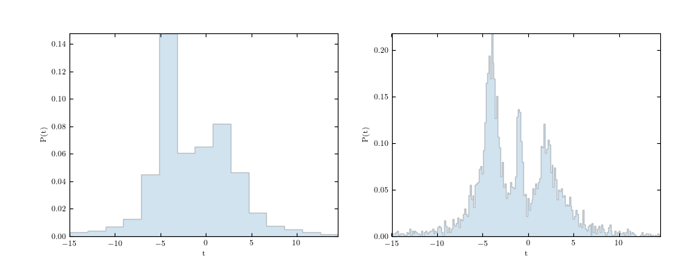
#------------------------------------------------------------
# First figure: show normal histogram binning
fig = plt.figure(figsize=(10, 4))
fig.subplots_adjust(left=0.1, right=0.95, bottom=0.15)
ax1 = fig.add_subplot(121)
ax1.hist(t, bins=15, histtype='stepfilled', alpha=0.2, density=True)
ax1.set_xlabel('t')
ax1.set_ylabel('P(t)')
ax2 = fig.add_subplot(122)
ax2.hist(t, bins=200, histtype='stepfilled', alpha=0.2, density=True)
ax2.set_xlabel('t')
ax2.set_ylabel('P(t)')
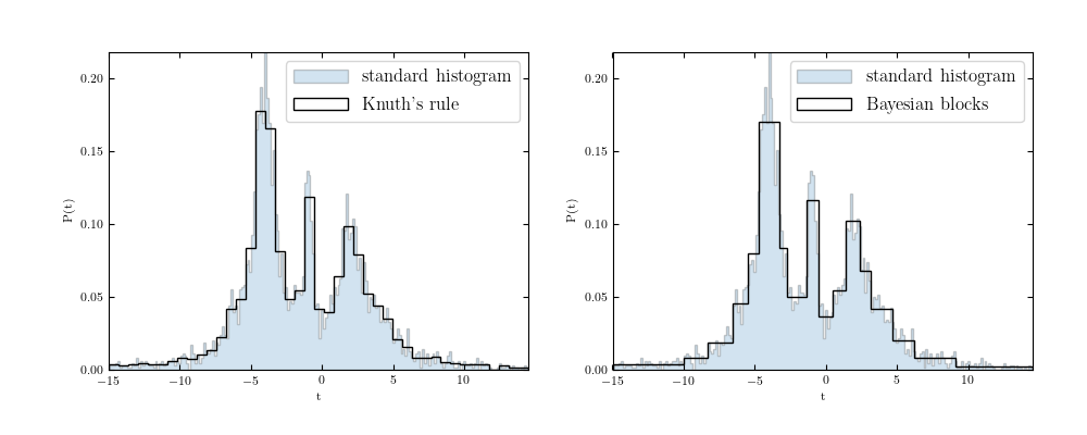
#------------------------------------------------------------
# Second & Third figure: Knuth bins & Bayesian Blocks
fig = plt.figure(figsize=(10, 4))
fig.subplots_adjust(left=0.1, right=0.95, bottom=0.15)
for bins, title, subplot in zip(['knuth', 'blocks'],
["Knuth's rule", 'Bayesian blocks'],
[121, 122]):
ax = fig.add_subplot(subplot)
# plot a standard histogram in the background, with alpha transparency
hist(t, bins=200, histtype='stepfilled',
alpha=0.2, density=True, label='standard histogram')
# plot an adaptive-width histogram on top
hist(t, bins=bins, ax=ax, color='black',
histtype='step', density=True, label=title)
ax.legend(prop=dict(size=12))
ax.set_xlabel('t')
ax.set_ylabel('P(t)')
plt.show()