SDSS Line-ratio Diagrams
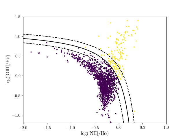
This shows how to plot line-ratio diagrams for the SDSS spectra. These diagrams are often called BPT plots 1, Osterbrock diagrams 2, or Kewley diagrams 3. The location of the dividing line is taken from from Kewley et al 2001.
References
- 1
Baldwin, J. A.; Phillips, M. M.; Terlevich, R. (1981) http://adsabs.harvard.edu/abs/1981PASP…93….5B
- 2
Osterbrock, D. E.; De Robertis, M. M. (1985) http://adsabs.harvard.edu/abs/1985PASP…97.1129O
- 3
Kewley, L. J. et al. (2001) http://adsabs.harvard.edu/abs/2001ApJ…556..121K
# Author: Jake VanderPlas <vanderplas@astro.washington.edu>
# License: BSD
#   The figure is an example from astroML: see http://astroML.github.com
import numpy as np
from matplotlib import pyplot as plt

from astroML.datasets import fetch_sdss_corrected_spectra
from astroML.datasets.tools.sdss_fits import log_OIII_Hb_NII

data = fetch_sdss_corrected_spectra()

i = np.where((data['lineindex_cln'] == 4) | (data['lineindex_cln'] == 5))

plt.scatter(data['log_NII_Ha'][i], data['log_OIII_Hb'][i],
            c=data['lineindex_cln'][i], s=9, lw=0)

NII = np.linspace(-2.0, 0.35)
plt.plot(NII, log_OIII_Hb_NII(NII), '-k')
plt.plot(NII, log_OIII_Hb_NII(NII, 0.1), '--k')
plt.plot(NII, log_OIII_Hb_NII(NII, -0.1), '--k')
plt.xlim(-2.0, 1.0)
plt.ylim(-1.2, 1.5)

plt.xlabel(r'$\mathrm{log([NII]/H\alpha)}$', fontsize='large')
plt.ylabel(r'$\mathrm{log([OIII]/H\beta)}$', fontsize='large')
plt.show()