NASA Sloan Atlas
This shows some visualizations of the data from the NASA SDSS Atlas

# Author: Jake VanderPlas <vanderplas@astro.washington.edu>
# License: BSD
# The figure is an example from astroML: see http://astroML.github.com
import numpy as np
from matplotlib import pyplot as plt
from astropy.visualization import hist
from astroML.datasets import fetch_nasa_atlas
data = fetch_nasa_atlas()
#------------------------------------------------------------
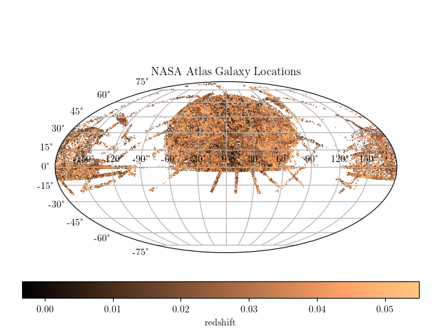
# plot the RA/DEC in an area-preserving projection
RA = data['RA']
DEC = data['DEC']
# convert coordinates to degrees
RA -= 180
RA *= np.pi / 180
DEC *= np.pi / 180
ax = plt.axes(projection='mollweide')
plt.scatter(RA, DEC, s=1, c=data['Z'], cmap=plt.cm.copper,
edgecolors='none', linewidths=0)
plt.grid(True)
plt.title('NASA Atlas Galaxy Locations')
cb = plt.colorbar(cax=plt.axes([0.05, 0.1, 0.9, 0.05]),
orientation='horizontal',
ticks=np.linspace(0, 0.05, 6))
cb.set_label('redshift')
#------------------------------------------------------------
# plot the r vs u-r color-magnitude diagram
absmag = data['ABSMAG']
u = absmag[:, 2]
r = absmag[:, 4]
plt.figure()
ax = plt.axes()
plt.scatter(u - r, r, s=1, lw=0, c=data['Z'], cmap=plt.cm.copper)
plt.colorbar(ticks=np.linspace(0, 0.05, 6)).set_label('redshift')
plt.xlim(0, 3.5)
plt.ylim(-10, -24)
plt.xlabel('u-r')
plt.ylabel('r')
#------------------------------------------------------------
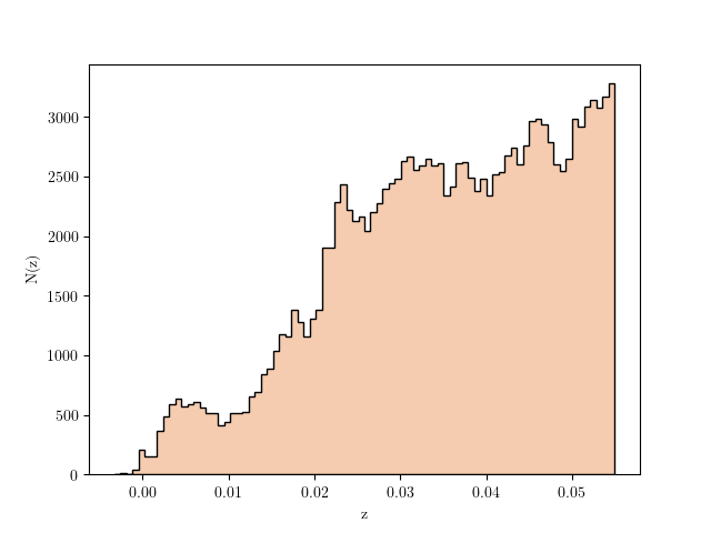
# plot a histogram of the redshift
plt.figure()
hist(data['Z'], bins='knuth',
histtype='stepfilled', ec='k', fc='#F5CCB0')
plt.xlabel('z')
plt.ylabel('N(z)')
plt.show()