Mixture Model of SDSS Great Wall

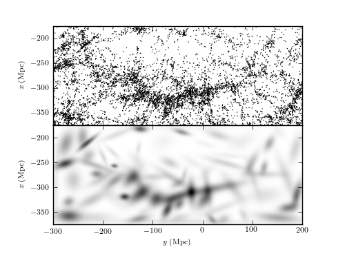
Figure 6.7

A two-dimensional mixture of 100 Gaussians (bottom) used to estimate the number density distribution of galaxies within the SDSS Great Wall (top). Compare to figures 6.3 and 6.4, where the density for the same distribution is computed using both kernel density and nearest-neighbor-based estimates.

Code output:

@pickle_results: using precomputed results from 'great_wall_GMM.pkl'

Python source code:

# Author: Jake VanderPlas
# License: BSD
#   The figure produced by this code is published in the textbook
#   "Statistics, Data Mining, and Machine Learning in Astronomy" (2013)
#   For more information, see http://astroML.github.com
#   To report a bug or issue, use the following forum:
#    https://groups.google.com/forum/#!forum/astroml-general
import numpy as np
from matplotlib import pyplot as plt

from sklearn.mixture import GMM
from astroML.datasets import fetch_great_wall
from astroML.decorators import pickle_results

#----------------------------------------------------------------------
# This function adjusts matplotlib settings for a uniform feel in the textbook.
# Note that with usetex=True, fonts are rendered with LaTeX.  This may
# result in an error if LaTeX is not installed on your system.  In that case,
# you can set usetex to False.
from astroML.plotting import setup_text_plots
setup_text_plots(fontsize=8, usetex=True)

#------------------------------------------------------------
# load great wall data
X = fetch_great_wall()


#------------------------------------------------------------
# Create a function which will save the results to a pickle file
#  for large number of clusters, computation will take a long time!
@pickle_results('great_wall_GMM.pkl')
def compute_GMM(n_clusters, n_iter=1000, min_covar=3, covariance_type='full'):
    clf = GMM(n_clusters, covariance_type=covariance_type,
              n_iter=n_iter, min_covar=min_covar)
    clf.fit(X)
    print "converged:", clf.converged_
    return clf

#------------------------------------------------------------
# Compute a grid on which to evaluate the result
Nx = 100
Ny = 250
xmin, xmax = (-375, -175)
ymin, ymax = (-300, 200)

Xgrid = np.vstack(map(np.ravel, np.meshgrid(np.linspace(xmin, xmax, Nx),
                                            np.linspace(ymin, ymax, Ny)))).T

#------------------------------------------------------------
# Compute the results
#
# we'll use 100 clusters.  In practice, one should cross-validate
# with AIC and BIC to settle on the correct number of clusters.
clf = compute_GMM(n_clusters=100)
log_dens = clf.score(Xgrid).reshape(Ny, Nx)

#------------------------------------------------------------
# Plot the results
fig = plt.figure(figsize=(5, 3.75))
fig.subplots_adjust(hspace=0, left=0.08, right=0.95, bottom=0.13, top=0.9)

ax = fig.add_subplot(211, aspect='equal')
ax.scatter(X[:, 1], X[:, 0], s=1, lw=0, c='k')

ax.set_xlim(ymin, ymax)
ax.set_ylim(xmin, xmax)

ax.xaxis.set_major_formatter(plt.NullFormatter())
plt.ylabel(r'$x\ {\rm (Mpc)}$')

ax = fig.add_subplot(212, aspect='equal')
ax.imshow(np.exp(log_dens.T), origin='lower', cmap=plt.cm.binary,
          extent=[ymin, ymax, xmin, xmax])
ax.set_xlabel(r'$y\ {\rm (Mpc)}$')
ax.set_ylabel(r'$x\ {\rm (Mpc)}$')

plt.show()

[download source: fig_great_wall_GMM.py]