EM example: Gaussian Mixture Models

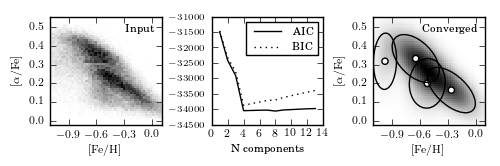
Figure 6.6

A two-dimensional mixture of Gaussians for the stellar metallicity data. The left panel shows the number density of stars as a function of two measures of their chemical composition: metallicity ([Fe/H]) and alpha-element abundance ([alpha/Fe]). The right panel shows the density estimated using mixtures of Gaussians together with the positions and covariances (2-sigma levels) of those Gaussians. The center panel compares the information criteria AIC and BIC (see Sections 4.3.2 and 5.4.3).

Code output:

@pickle_results: using precomputed results from 'GMM_metallicity.pkl'
best fit converged: True
BIC: n_components =  4

Python source code:

# Author: Jake VanderPlas
# License: BSD
#   The figure produced by this code is published in the textbook
#   "Statistics, Data Mining, and Machine Learning in Astronomy" (2013)
#   For more information, see http://astroML.github.com
#   To report a bug or issue, use the following forum:
#    https://groups.google.com/forum/#!forum/astroml-general
import numpy as np
from matplotlib import pyplot as plt
from scipy.stats import norm

from sklearn.mixture import GMM

from astroML.datasets import fetch_sdss_sspp
from astroML.decorators import pickle_results
from astroML.plotting.tools import draw_ellipse

#----------------------------------------------------------------------
# This function adjusts matplotlib settings for a uniform feel in the textbook.
# Note that with usetex=True, fonts are rendered with LaTeX.  This may
# result in an error if LaTeX is not installed on your system.  In that case,
# you can set usetex to False.
from astroML.plotting import setup_text_plots
setup_text_plots(fontsize=8, usetex=True)

#------------------------------------------------------------
# Get the Segue Stellar Parameters Pipeline data
data = fetch_sdss_sspp(cleaned=True)
X = np.vstack([data['FeH'], data['alphFe']]).T

# truncate dataset for speed
X = X[::5]

#------------------------------------------------------------
# Compute GMM models & AIC/BIC
N = np.arange(1, 14)


@pickle_results("GMM_metallicity.pkl")
def compute_GMM(N, covariance_type='full', n_iter=1000):
    models = [None for n in N]
    for i in range(len(N)):
        print N[i]
        models[i] = GMM(n_components=N[i], n_iter=n_iter,
                        covariance_type=covariance_type)
        models[i].fit(X)
    return models

models = compute_GMM(N)

AIC = [m.aic(X) for m in models]
BIC = [m.bic(X) for m in models]

i_best = np.argmin(BIC)
gmm_best = models[i_best]
print "best fit converged:", gmm_best.converged_
print "BIC: n_components =  %i" % N[i_best]

#------------------------------------------------------------
# compute 2D density
FeH_bins = 51
alphFe_bins = 51
H, FeH_bins, alphFe_bins = np.histogram2d(data['FeH'], data['alphFe'],
                                          (FeH_bins, alphFe_bins))

Xgrid = np.array(map(np.ravel,
                     np.meshgrid(0.5 * (FeH_bins[:-1]
                                        + FeH_bins[1:]),
                                 0.5 * (alphFe_bins[:-1]
                                        + alphFe_bins[1:])))).T
log_dens = gmm_best.score(Xgrid).reshape((51, 51))

#------------------------------------------------------------
# Plot the results
fig = plt.figure(figsize=(5, 1.66))
fig.subplots_adjust(wspace=0.45,
                    bottom=0.25, top=0.9,
                    left=0.1, right=0.97)

# plot density
ax = fig.add_subplot(131)
ax.imshow(H.T, origin='lower', interpolation='nearest', aspect='auto',
          extent=[FeH_bins[0], FeH_bins[-1],
                  alphFe_bins[0], alphFe_bins[-1]],
          cmap=plt.cm.binary)
ax.set_xlabel(r'$\rm [Fe/H]$')
ax.set_ylabel(r'$\rm [\alpha/Fe]$')
ax.xaxis.set_major_locator(plt.MultipleLocator(0.3))
ax.set_xlim(-1.101, 0.101)
ax.text(0.93, 0.93, "Input",
        va='top', ha='right', transform=ax.transAxes)

# plot AIC/BIC
ax = fig.add_subplot(132)
ax.plot(N, AIC, '-k', label='AIC')
ax.plot(N, BIC, ':k', label='BIC')
ax.legend(loc=1)
ax.set_xlabel('N components')
plt.setp(ax.get_yticklabels(), fontsize=7)

# plot best configurations for AIC and BIC
ax = fig.add_subplot(133)
ax.imshow(np.exp(log_dens),
          origin='lower', interpolation='nearest', aspect='auto',
          extent=[FeH_bins[0], FeH_bins[-1],
                  alphFe_bins[0], alphFe_bins[-1]],
          cmap=plt.cm.binary)

ax.scatter(gmm_best.means_[:, 0], gmm_best.means_[:, 1], c='w')
for mu, C, w in zip(gmm_best.means_, gmm_best.covars_, gmm_best.weights_):
    draw_ellipse(mu, C, scales=[1.5], ax=ax, fc='none', ec='k')

ax.text(0.93, 0.93, "Converged",
        va='top', ha='right', transform=ax.transAxes)

ax.set_xlim(-1.101, 0.101)
ax.set_ylim(alphFe_bins[0], alphFe_bins[-1])
ax.xaxis.set_major_locator(plt.MultipleLocator(0.3))
ax.set_xlabel(r'$\rm [Fe/H]$')
ax.set_ylabel(r'$\rm [\alpha/Fe]$')

plt.show()

[download source: fig_EM_metallicity.py]