Comparison of 1D Density Estimators

Figure 6.8

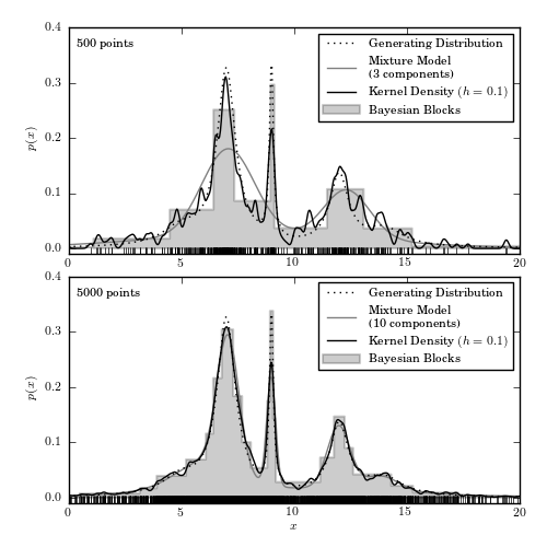
A comparison of different density estimation methods for two simulated one-dimensional data sets (same as in figure 6.5). Density estimators are Bayesian blocks (Section 5.7.2), KDE (Section 6.1.1), and a Gaussian mixture model. In the latter, the optimal number of Gaussian components is chosen using the BIC (eq. 5.35). In the top panel, GMM solution has three components but one of the components has a very large width and effectively acts as a nearly flat background.

Code output:

WARNING: DeprecationWarning: Function eval is deprecated; GMM.eval was renamed to GMM.score_samples in 0.14 and will be removed in 0.16. [sklearn.utils]
WARNING: DeprecationWarning: Function eval is deprecated; GMM.eval was renamed to GMM.score_samples in 0.14 and will be removed in 0.16. [sklearn.utils]

Python source code:

# Author: Jake VanderPlas
# License: BSD
#   The figure produced by this code is published in the textbook
#   "Statistics, Data Mining, and Machine Learning in Astronomy" (2013)
#   For more information, see http://astroML.github.com
#   To report a bug or issue, use the following forum:
#    https://groups.google.com/forum/#!forum/astroml-general
import numpy as np
from matplotlib import pyplot as plt
from scipy import stats

from astroML.plotting import hist
from sklearn.mixture import GMM

# Scikit-learn 0.14 added sklearn.neighbors.KernelDensity, which is a very
# fast kernel density estimator based on a KD Tree.  We'll use this if
# available (and raise a warning if it isn't).
try:
    from sklearn.neighbors import KernelDensity
    use_sklearn_KDE = True
except:
    import warnings
    warnings.warn("KDE will be removed in astroML version 0.3.  Please "
                  "upgrade to scikit-learn 0.14+ and use "
                  "sklearn.neighbors.KernelDensity.", DeprecationWarning)
    from astroML.density_estimation import KDE
    use_sklearn_KDE = False


#----------------------------------------------------------------------
# This function adjusts matplotlib settings for a uniform feel in the textbook.
# Note that with usetex=True, fonts are rendered with LaTeX.  This may
# result in an error if LaTeX is not installed on your system.  In that case,
# you can set usetex to False.
from astroML.plotting import setup_text_plots
setup_text_plots(fontsize=8, usetex=True)

#------------------------------------------------------------
# Generate our data: a mix of several Cauchy distributions
#  this is the same data used in the Bayesian Blocks figure
np.random.seed(0)
N = 10000
mu_gamma_f = [(5, 1.0, 0.1),
              (7, 0.5, 0.5),
              (9, 0.1, 0.1),
              (12, 0.5, 0.2),
              (14, 1.0, 0.1)]
true_pdf = lambda x: sum([f * stats.cauchy(mu, gamma).pdf(x)
                          for (mu, gamma, f) in mu_gamma_f])
x = np.concatenate([stats.cauchy(mu, gamma).rvs(int(f * N))
                    for (mu, gamma, f) in mu_gamma_f])
np.random.shuffle(x)
x = x[x > -10]
x = x[x < 30]

#------------------------------------------------------------
# plot the results
fig = plt.figure(figsize=(5, 5))
fig.subplots_adjust(bottom=0.08, top=0.95, right=0.95, hspace=0.1)
N_values = (500, 5000)
subplots = (211, 212)
k_values = (10, 100)

for N, k, subplot in zip(N_values, k_values, subplots):
    ax = fig.add_subplot(subplot)
    xN = x[:N]
    t = np.linspace(-10, 30, 1000)

    # Compute density with KDE
    if use_sklearn_KDE:
        kde = KernelDensity(0.1, kernel='gaussian')
        kde.fit(xN[:, None])
        dens_kde = np.exp(kde.score_samples(t[:, None]))
    else:
        kde = KDE('gaussian', h=0.1).fit(xN[:, None])
        dens_kde = kde.eval(t[:, None]) / N

    # Compute density via Gaussian Mixtures
    # we'll try several numbers of clusters
    n_components = np.arange(3, 16)
    gmms = [GMM(n_components=n).fit(xN) for n in n_components]
    BICs = [gmm.bic(xN) for gmm in gmms]
    i_min = np.argmin(BICs)
    t = np.linspace(-10, 30, 1000)
    logprob, responsibilities = gmms[i_min].eval(t)

    # plot the results
    ax.plot(t, true_pdf(t), ':', color='black', zorder=3,
            label="Generating Distribution")
    ax.plot(xN, -0.005 * np.ones(len(xN)), '|k', lw=1.5)
    hist(xN, bins='blocks', ax=ax, normed=True, zorder=1,
         histtype='stepfilled', lw=1.5, color='k', alpha=0.2,
         label="Bayesian Blocks")
    ax.plot(t, np.exp(logprob), '-', color='gray',
            label="Mixture Model\n(%i components)" % n_components[i_min])
    ax.plot(t, dens_kde, '-', color='black', zorder=3,
            label="Kernel Density $(h=0.1)$")

    # label the plot
    ax.text(0.02, 0.95, "%i points" % N, ha='left', va='top',
            transform=ax.transAxes)
    ax.set_ylabel('$p(x)$')
    ax.legend(loc='upper right')

    if subplot == 212:
        ax.set_xlabel('$x$')

    ax.set_xlim(0, 20)
    ax.set_ylim(-0.01, 0.4001)

plt.show()

[download source: fig_GMM_density_estimation.py]