MCMC Model Comparison
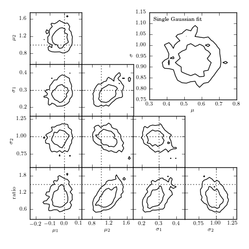
Figure 5.24
The top-right panel shows the posterior pdf for mu and sigma for a single Gaussian fit to the data shown in figure 5.23. The remaining panels show the projections of the five-dimensional pdf for a Gaussian mixture model with two components. Contours are based on a 10,000 point MCMC chain.
[--------------   38%                  ] 3847 of 10000 complete in 0.5 sec
[-----------------75%--------          ] 7513 of 10000 complete in 1.0 sec
[-----------------100%-----------------] 10000 of 10000 complete in 1.3 sec
[                  2%                  ] 262 of 10000 complete in 0.5 sec
[-                 5%                  ] 524 of 10000 complete in 1.0 sec
[--                7%                  ] 781 of 10000 complete in 1.5 sec
[---              10%                  ] 1031 of 10000 complete in 2.0 sec
[----             12%                  ] 1282 of 10000 complete in 2.5 sec
[-----            15%                  ] 1533 of 10000 complete in 3.0 sec
[------           17%                  ] 1780 of 10000 complete in 3.5 sec
[-------          20%                  ] 2026 of 10000 complete in 4.0 sec
[--------         22%                  ] 2277 of 10000 complete in 4.5 sec
[---------        25%                  ] 2525 of 10000 complete in 5.0 sec
[----------       27%                  ] 2780 of 10000 complete in 5.5 sec
[-----------      30%                  ] 3030 of 10000 complete in 6.0 sec
[------------     32%                  ] 3277 of 10000 complete in 6.5 sec
[-------------    35%                  ] 3527 of 10000 complete in 7.0 sec
[--------------   37%                  ] 3780 of 10000 complete in 7.5 sec
[---------------  40%                  ] 4022 of 10000 complete in 8.0 sec
[---------------- 42%                  ] 4272 of 10000 complete in 8.5 sec
[-----------------45%                  ] 4518 of 10000 complete in 9.0 sec
[-----------------47%                  ] 4769 of 10000 complete in 9.5 sec
[-----------------50%                  ] 5022 of 10000 complete in 10.0 sec
[-----------------52%                  ] 5278 of 10000 complete in 10.5 sec
[-----------------55%                  ] 5523 of 10000 complete in 11.0 sec
[-----------------57%-                 ] 5776 of 10000 complete in 11.5 sec
[-----------------60%--                ] 6021 of 10000 complete in 12.0 sec
[-----------------62%---               ] 6274 of 10000 complete in 12.5 sec
[-----------------65%----              ] 6520 of 10000 complete in 13.0 sec
[-----------------67%-----             ] 6769 of 10000 complete in 13.5 sec
[-----------------70%------            ] 7013 of 10000 complete in 14.0 sec
[-----------------72%-------           ] 7262 of 10000 complete in 14.5 sec
[-----------------75%--------          ] 7511 of 10000 complete in 15.0 sec
[-----------------77%---------         ] 7763 of 10000 complete in 15.5 sec
[-----------------80%----------        ] 8013 of 10000 complete in 16.0 sec
[-----------------82%-----------       ] 8263 of 10000 complete in 16.5 sec
[-----------------85%------------      ] 8515 of 10000 complete in 17.0 sec
[-----------------87%-------------     ] 8768 of 10000 complete in 17.5 sec
[-----------------90%--------------    ] 9016 of 10000 complete in 18.0 sec
[-----------------92%---------------   ] 9266 of 10000 complete in 18.5 sec
[-----------------95%----------------  ] 9514 of 10000 complete in 19.0 sec
[-----------------97%----------------- ] 9768 of 10000 complete in 19.5 sec
[-----------------100%-----------------] 10000 of 10000 complete in 20.0 sec
# Author: Jake VanderPlas
# License: BSD
#   The figure produced by this code is published in the textbook
#   "Statistics, Data Mining, and Machine Learning in Astronomy" (2013)
#   For more information, see http://astroML.github.com
#   To report a bug or issue, use the following forum:
#    https://groups.google.com/forum/#!forum/astroml-general
import numpy as np
from matplotlib import pyplot as plt

from scipy.special import gamma
from scipy.stats import norm
from sklearn.neighbors import BallTree
from astroML.density_estimation import GaussianMixture1D
from astroML.plotting import plot_mcmc
# hack to fix an import issue in older versions of pymc
import scipy
scipy.derivative = scipy.misc.derivative
import pymc

#----------------------------------------------------------------------
# This function adjusts matplotlib settings for a uniform feel in the textbook.
# Note that with usetex=True, fonts are rendered with LaTeX.  This may
# result in an error if LaTeX is not installed on your system.  In that case,
# you can set usetex to False.
from astroML.plotting import setup_text_plots
setup_text_plots(fontsize=8, usetex=True)


def get_logp(S, model):
    """compute log(p) given a pyMC model"""
    M = pymc.MAP(model)
    traces = np.array([S.trace(s)[:] for s in S.stochastics])
    logp = np.zeros(traces.shape[1])
    for i in range(len(logp)):
        logp[i] = -M.func(traces[:, i])
    return logp


def estimate_bayes_factor(traces, logp, r=0.05, return_list=False):
    """Estimate the bayes factor using the local density of points"""
    D, N = traces.shape

    # compute volume of a D-dimensional sphere of radius r
    Vr = np.pi ** (0.5 * D) / gamma(0.5 * D + 1) * (r ** D)

    # use neighbor count within r as a density estimator
    bt = BallTree(traces.T)
    count = bt.query_radius(traces.T, r=r, count_only=True)

    BF = logp + np.log(N) + np.log(Vr) - np.log(count)

    if return_list:
        return BF
    else:
        p25, p50, p75 = np.percentile(BF, [25, 50, 75])
        return p50, 0.7413 * (p75 - p25)


#------------------------------------------------------------
# Generate the data
mu1_in = 0
sigma1_in = 0.3
mu2_in = 1
sigma2_in = 1
ratio_in = 1.5
N = 200

np.random.seed(10)
gm = GaussianMixture1D([mu1_in, mu2_in],
                       [sigma1_in, sigma2_in],
                       [ratio_in, 1])
x_sample = gm.sample(N)

#------------------------------------------------------------
# Set up pyMC model: single gaussian
#  2 parameters: (mu, sigma)
M1_mu = pymc.Uniform('M1_mu', -5, 5, value=0)
M1_log_sigma = pymc.Uniform('M1_log_sigma', -10, 10, value=0)


@pymc.deterministic
def M1_sigma(M1_log_sigma=M1_log_sigma):
    return np.exp(M1_log_sigma)


@pymc.deterministic
def M1_tau(M1_sigma=M1_sigma):
    return 1. / M1_sigma ** 2

M1 = pymc.Normal('M1', M1_mu, M1_tau, observed=True, value=x_sample)
model1 = dict(M1_mu=M1_mu, M1_log_sigma=M1_log_sigma,
              M1_sigma=M1_sigma,
              M1_tau=M1_tau, M1=M1)


#------------------------------------------------------------
# Set up pyMC model: double gaussian
#  5 parameters: (mu1, mu2, sigma1, sigma2, ratio)

def doublegauss_like(x, mu1, mu2, sigma1, sigma2, ratio):
    """log-likelihood for double gaussian"""
    r1 = ratio / (1. + ratio)
    r2 = 1 - r1
    L = r1 * norm(mu1, sigma1).pdf(x) + r2 * norm(mu2, sigma2).pdf(x)
    L[L == 0] = 1E-16  # prevent divide-by-zero error
    logL = np.log(L).sum()
    if np.isinf(logL):
        raise pymc.ZeroProbability
    else:
        return logL


def rdoublegauss(mu1, mu2, sigma1, sigma2, ratio, size=None):
    """random variable from double gaussian"""
    r1 = ratio / (1. + ratio)
    r2 = 1 - r1
    R = np.asarray(np.random.random(size))

    Rshape = R.shape
    R = np.atleast1d(R)

    mask1 = (R < r1)
    mask2 = ~mask1
    N1 = mask1.sum()
    N2 = R.size - N1

    R[mask1] = norm(mu1, sigma1).rvs(N1)
    R[mask2] = norm(mu2, sigma2).rvs(N2)

    return R.reshape(Rshape)

DoubleGauss = pymc.stochastic_from_dist('doublegauss',
                                        logp=doublegauss_like,
                                        random=rdoublegauss,
                                        dtype=np.float,
                                        mv=True)

# set up our Stochastic variables, mu1, mu2, sigma1, sigma2, ratio
M2_mu1 = pymc.Uniform('M2_mu1', -5, 5, value=0)
M2_mu2 = pymc.Uniform('M2_mu2', -5, 5, value=1)

M2_log_sigma1 = pymc.Uniform('M2_log_sigma1', -10, 10, value=0)
M2_log_sigma2 = pymc.Uniform('M2_log_sigma2', -10, 10, value=0)


@pymc.deterministic
def M2_sigma1(M2_log_sigma1=M2_log_sigma1):
    return np.exp(M2_log_sigma1)


@pymc.deterministic
def M2_sigma2(M2_log_sigma2=M2_log_sigma2):
    return np.exp(M2_log_sigma2)

M2_ratio = pymc.Uniform('M2_ratio', 1E-3, 1E3, value=1)

M2 = DoubleGauss('M2', M2_mu1, M2_mu2, M2_sigma1, M2_sigma2, M2_ratio,
                 observed=True, value=x_sample)

model2 = dict(M2_mu1=M2_mu1, M2_mu2=M2_mu2,
              M2_log_sigma1=M2_log_sigma1, M2_log_sigma2=M2_log_sigma2,
              M2_sigma1=M2_sigma1, M2_sigma2=M2_sigma2,
              M2_ratio=M2_ratio, M2=M2)


#------------------------------------------------------------
# Set up MCMC sampling
def compute_MCMC_models(Niter=10000, burn=1000, rseed=0):
    pymc.numpy.random.seed(rseed)

    S1 = pymc.MCMC(model1)
    S1.sample(iter=Niter, burn=burn)
    trace1 = np.vstack([S1.trace('M1_mu')[:],
                        S1.trace('M1_sigma')[:]])
    logp1 = get_logp(S1, model1)

    S2 = pymc.MCMC(model2)
    S2.sample(iter=Niter, burn=burn)
    trace2 = np.vstack([S2.trace('M2_mu1')[:],
                        S2.trace('M2_mu2')[:],
                        S2.trace('M2_sigma1')[:],
                        S2.trace('M2_sigma2')[:],
                        S2.trace('M2_ratio')[:]])
    logp2 = get_logp(S2, model2)

    return trace1, logp1, trace2, logp2

trace1, logp1, trace2, logp2 = compute_MCMC_models()


#------------------------------------------------------------
# Compute Odds ratio with density estimation technique
BF1, dBF1 = estimate_bayes_factor(trace1, logp1, r=0.02)
BF2, dBF2 = estimate_bayes_factor(trace2, logp2, r=0.05)


#------------------------------------------------------------
# Plot the results
fig = plt.figure(figsize=(5, 5))

labels = [r'$\mu_1$',
          r'$\mu_2$',
          r'$\sigma_1$',
          r'$\sigma_2$',
          r'${\rm ratio}$']

true_values = [mu1_in,
               mu2_in,
               sigma1_in,
               sigma2_in,
               ratio_in]

limits = [(-0.24, 0.12),
          (0.55, 1.75),
          (0.15, 0.45),
          (0.55, 1.3),
          (0.25, 2.1)]

# we assume mu1 < mu2, but the results may be switched
#  due to the symmetry of the problem.  If so, switch back
if np.median(trace2[0]) > np.median(trace2[1]):
    trace2 = trace2[[1, 0, 3, 2, 4], :]
    N2_norm_mu = N2.mu[N2.M2_mu2, N2.M2_mu1,
                       N2.M2_sigma2, N2.M2_sigma1, N2.M2_ratio]
    N2_norm_Sig = N2.C[N2.M2_mu2, N2.M2_mu1,
                       N2.M2_sigma2, N2.M2_sigma1, N2.M2_ratio]

# Plot the simple 2-component model
ax, = plot_mcmc(trace1, fig=fig, bounds=[0.6, 0.6, 0.95, 0.95],
                limits=[(0.3, 0.8), (0.75, 1.15)],
                labels=[r'$\mu$', r'$\sigma$'], colors='k')

ax.text(0.05, 0.95, "Single Gaussian fit", va='top', ha='left',
        transform=ax.transAxes)

# Plot the 5-component model
ax_list = plot_mcmc(trace2, limits=limits, labels=labels,
                    true_values=true_values, fig=fig,
                    bounds=(0.12, 0.12, 0.95, 0.95),
                    colors='k')
for ax in ax_list:
    for axis in [ax.xaxis, ax.yaxis]:
        axis.set_major_locator(plt.MaxNLocator(4))

plt.show()