Histogram for Double-gaussian model test

Figure 5.23

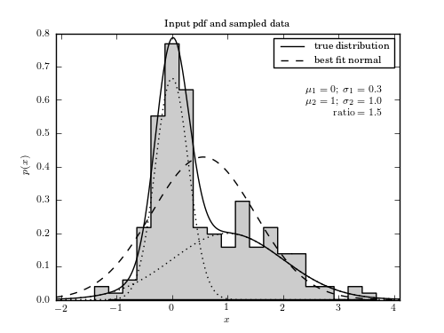
A sample of 200 points drawn from a Gaussian mixture model used to illustrate model selection with MCMC.

Code output:

WARNING: DeprecationWarning: Function eval is deprecated; GMM.eval was renamed to GMM.score_samples in 0.14 and will be removed in 0.16. [sklearn.utils]
WARNING: DeprecationWarning: Function eval is deprecated; GMM.eval was renamed to GMM.score_samples in 0.14 and will be removed in 0.16. [sklearn.utils]

Python source code:

# Author: Jake VanderPlas
# License: BSD
#   The figure produced by this code is published in the textbook
#   "Statistics, Data Mining, and Machine Learning in Astronomy" (2013)
#   For more information, see http://astroML.github.com
#   To report a bug or issue, use the following forum:
#    https://groups.google.com/forum/#!forum/astroml-general
import numpy as np
from matplotlib import pyplot as plt
from scipy.stats import norm
from astroML.density_estimation import GaussianMixture1D

#----------------------------------------------------------------------
# This function adjusts matplotlib settings for a uniform feel in the textbook.
# Note that with usetex=True, fonts are rendered with LaTeX.  This may
# result in an error if LaTeX is not installed on your system.  In that case,
# you can set usetex to False.
from astroML.plotting import setup_text_plots
setup_text_plots(fontsize=8, usetex=True)

#------------------------------------------------------------
# Generate the data
mu1_in = 0
sigma1_in = 0.3
mu2_in = 1
sigma2_in = 1
ratio_in = 1.5
N = 200

np.random.seed(10)
gm = GaussianMixture1D([mu1_in, mu2_in],
                       [sigma1_in, sigma2_in],
                       [ratio_in, 1])
x_sample = gm.sample(N)

#------------------------------------------------------------
# Get the MLE fit for a single gaussian
sample_mu = np.mean(x_sample)
sample_std = np.std(x_sample, ddof=1)

#------------------------------------------------------------
# Plot the sampled data
fig, ax = plt.subplots(figsize=(5, 3.75))

ax.hist(x_sample, 20, histtype='stepfilled', normed=True, fc='#CCCCCC')
x = np.linspace(-2.1, 4.1, 1000)

factor1 = ratio_in / (1. + ratio_in)
factor2 = 1. / (1. + ratio_in)

ax.plot(x, gm.pdf(x), '-k', label='true distribution')
ax.plot(x, gm.pdf_individual(x), ':k')

ax.plot(x, norm.pdf(x, sample_mu, sample_std), '--k', label='best fit normal')

ax.legend(loc=1)

ax.set_xlim(-2.1, 4.1)

ax.set_xlabel('$x$')
ax.set_ylabel('$p(x)$')
ax.set_title('Input pdf and sampled data')
ax.text(0.95, 0.80, ('$\mu_1 = 0;\ \sigma_1=0.3$\n'
                     '$\mu_2=1;\ \sigma_2=1.0$\n'
                     '$\mathrm{ratio}=1.5$'),
        transform=ax.transAxes, ha='right', va='top')
plt.show()

[download source: fig_model_comparison_hist.py]