Gaussian Distribution with Gaussian Errors

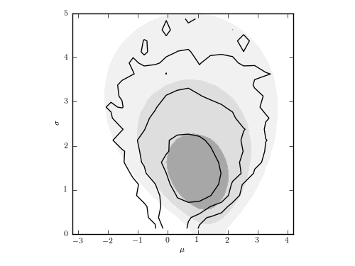
Figure 5.25

The posterior pdf for mu and sigma for a Gaussian distribution with heteroscedastic errors. This is the same data set as used in figure 5.7, but here each measurement error is assumed unknown, treated as a model parameter with a scale-invariant prior, and marginalized over to obtain the distribution of mu and sigma shown by contours. For comparison, the posterior pdf from figure 5.7 is shown by shaded contours.

Code output:

[--                7%                  ] 1842 of 25000 complete in 0.5 sec
[----             12%                  ] 3085 of 25000 complete in 1.0 sec
[-------          18%                  ] 4701 of 25000 complete in 1.5 sec
[---------        24%                  ] 6017 of 25000 complete in 2.0 sec
[-----------      29%                  ] 7426 of 25000 complete in 2.5 sec
[-------------    36%                  ] 9161 of 25000 complete in 3.0 sec
[---------------- 42%                  ] 10596 of 25000 complete in 3.5 sec
[-----------------49%                  ] 12291 of 25000 complete in 4.0 sec
[-----------------55%-                 ] 13933 of 25000 complete in 4.5 sec
[-----------------62%---               ] 15652 of 25000 complete in 5.0 sec
[-----------------69%------            ] 17312 of 25000 complete in 5.5 sec
[-----------------76%--------          ] 19065 of 25000 complete in 6.0 sec
[-----------------83%-----------       ] 20764 of 25000 complete in 6.5 sec
[-----------------90%--------------    ] 22548 of 25000 complete in 7.0 sec
[-----------------96%----------------  ] 24246 of 25000 complete in 7.5 sec
[-----------------100%-----------------] 25000 of 25000 complete in 7.7 sec

Python source code:

# Author: Jake VanderPlas
# License: BSD
#   The figure produced by this code is published in the textbook
#   "Statistics, Data Mining, and Machine Learning in Astronomy" (2013)
#   For more information, see http://astroML.github.com
#   To report a bug or issue, use the following forum:
#    https://groups.google.com/forum/#!forum/astroml-general
import numpy as np
from matplotlib import pyplot as plt

# Hack to fix import issue in older versions of pymc
import scipy
import scipy.misc
scipy.derivative = scipy.misc.derivative
import pymc

from astroML.plotting.mcmc import convert_to_stdev
from astroML.plotting import plot_mcmc

#----------------------------------------------------------------------
# This function adjusts matplotlib settings for a uniform feel in the textbook.
# Note that with usetex=True, fonts are rendered with LaTeX.  This may
# result in an error if LaTeX is not installed on your system.  In that case,
# you can set usetex to False.
from astroML.plotting import setup_text_plots
setup_text_plots(fontsize=8, usetex=True)


def gaussgauss_logL(xi, ei, mu, sigma):
    """Equation 5.22: gaussian likelihood"""
    ndim = len(np.broadcast(sigma, mu).shape)

    xi = xi.reshape(xi.shape + tuple(ndim * [1]))
    ei = ei.reshape(ei.shape + tuple(ndim * [1]))

    s2_e2 = sigma ** 2 + ei ** 2
    return -0.5 * np.sum(np.log(s2_e2) + (xi - mu) ** 2 / s2_e2, 0)


#------------------------------------------------------------
# Select the data
np.random.seed(5)
mu_true = 1.
sigma_true = 1.
N = 10
ei = 3 * np.random.random(N)
xi = np.random.normal(mu_true, np.sqrt(sigma_true ** 2 + ei ** 2))

#----------------------------------------------------------------------
# Set up MCMC for our model parameters: (mu, sigma, ei)
mu = pymc.Uniform('mu', -10, 10, value=0)
log_sigma = pymc.Uniform('log_sigma', -10, 10, value=0)
log_error = pymc.Uniform('log_error', -10, 10, value=np.zeros(N))


@pymc.deterministic
def sigma(log_sigma=log_sigma):
    return np.exp(log_sigma)


@pymc.deterministic
def error(log_error=log_error):
    return np.exp(log_error)


def gaussgauss_like(x, mu, sigma, error):
    """likelihood of gaussian with gaussian errors"""
    sig2 = sigma ** 2 + error ** 2
    x_mu2 = (x - mu) ** 2
    return -0.5 * np.sum(np.log(sig2) + x_mu2 / sig2)

GaussGauss = pymc.stochastic_from_dist('gaussgauss',
                                       logp=gaussgauss_like,
                                       dtype=np.float,
                                       mv=True)
M = GaussGauss('M', mu, sigma, error, observed=True, value=xi)

model = dict(mu=mu, log_sigma=log_sigma, sigma=sigma,
             log_error=log_error, error=error, M=M)

#------------------------------------------------------------
# perform the MCMC sampling
np.random.seed(0)
S = pymc.MCMC(model)
S.sample(iter=25000, burn=2000)

#------------------------------------------------------------
# Extract the MCMC traces
trace_mu = S.trace('mu')[:]
trace_sigma = S.trace('sigma')[:]

fig = plt.figure(figsize=(5, 3.75))
ax, = plot_mcmc([trace_mu, trace_sigma], fig=fig,
                limits=[(-3.2, 4.2), (0, 5)],
                bounds=(0.08, 0.12, 0.95, 0.95),
                labels=(r'$\mu$', r'$\sigma$'),
                levels=[0.683, 0.955, 0.997],
                colors='k')

#----------------------------------------------------------------------
# Compute and plot likelihood with known ei for comparison
# (Same as fig_likelihood_gaussgauss)
sigma = np.linspace(0.01, 5, 41)
mu = np.linspace(-3.2, 4.2, 41)

logL = gaussgauss_logL(xi, ei, mu, sigma[:, np.newaxis])
logL -= logL.max()

im = ax.contourf(mu, sigma, convert_to_stdev(logL),
                 levels=(0, 0.683, 0.955, 0.997),
                 cmap=plt.cm.binary_r, alpha=0.5)
im.set_clim(0, 1.1)

ax.set_xlabel(r'$\mu$')
ax.set_ylabel(r'$\sigma$')
ax.set_xlim(-3.2, 4.2)
ax.set_ylim(0, 5)

ax.set_aspect(1. / ax.get_data_ratio())

plt.show()

[download source: fig_gaussgauss_mcmc.py]