Finding a signal in a background

Figure 5.26

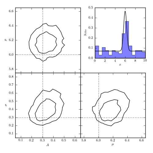
Fitting a model of a signal in an unknown background. The histogram in the top-right panel visualizes a sample drawn from a Gaussian signal plus a uniform background model given by eq. 5.83 and shown by the line. The remaining panels show projections of the three-dimensional posterior pdf, based on a 20,000 point MCMC chain.

Code output:

[--                7%                  ] 1931 of 25000 complete in 0.5 sec
[-----            14%                  ] 3698 of 25000 complete in 1.0 sec
[--------         21%                  ] 5342 of 25000 complete in 1.5 sec
[----------       27%                  ] 6859 of 25000 complete in 2.0 sec
[------------     33%                  ] 8408 of 25000 complete in 2.5 sec
[---------------  40%                  ] 10048 of 25000 complete in 3.0 sec
[-----------------46%                  ] 11670 of 25000 complete in 3.5 sec
[-----------------52%                  ] 13204 of 25000 complete in 4.0 sec
[-----------------59%--                ] 14757 of 25000 complete in 4.5 sec
[-----------------65%----              ] 16369 of 25000 complete in 5.0 sec
[-----------------71%-------           ] 17942 of 25000 complete in 5.5 sec
[-----------------78%---------         ] 19546 of 25000 complete in 6.0 sec
[-----------------83%-----------       ] 20989 of 25000 complete in 6.5 sec
[-----------------90%--------------    ] 22566 of 25000 complete in 7.0 sec
[-----------------96%----------------  ] 24106 of 25000 complete in 7.5 sec
[-----------------100%-----------------] 25000 of 25000 complete in 7.8 sec

Python source code:

# Author: Jake VanderPlas
# License: BSD
#   The figure produced by this code is published in the textbook
#   "Statistics, Data Mining, and Machine Learning in Astronomy" (2013)
#   For more information, see http://astroML.github.com
#   To report a bug or issue, use the following forum:
#    https://groups.google.com/forum/#!forum/astroml-general
import numpy as np
from matplotlib import pyplot as plt
from scipy import stats

# Hack to fix import issue in older versions of pymc
import scipy
import scipy.misc
scipy.derivative = scipy.misc.derivative
import pymc

from astroML.plotting import plot_mcmc

#----------------------------------------------------------------------
# This function adjusts matplotlib settings for a uniform feel in the textbook.
# Note that with usetex=True, fonts are rendered with LaTeX.  This may
# result in an error if LaTeX is not installed on your system.  In that case,
# you can set usetex to False.
from astroML.plotting import setup_text_plots
setup_text_plots(fontsize=8, usetex=True)

#----------------------------------------------------------------------
# Set up dataset: gaussian signal in a uniform background
np.random.seed(0)

N = 100

A_true = 0.3
W_true = 10
x0_true = 6
sigma_true = 0.3

signal = stats.norm(x0_true, sigma_true)
background = stats.uniform(0, W_true)

x = np.random.random(N)
i_sig = x < A_true
i_bg = ~i_sig
x[i_sig] = signal.rvs(np.sum(i_sig))
x[i_bg] = background.rvs(np.sum(i_bg))

#----------------------------------------------------------------------
# Set up MCMC sampling
A = pymc.Uniform('A', 0, 1, value=0.5)
x0 = pymc.Uniform('x0', 0, 10, value=5)
log_sigma = pymc.Uniform('log_sigma', -5, 5, value=0)


@pymc.deterministic
def sigma(log_sigma=log_sigma):
    return np.exp(log_sigma)


def sigbg_like(x, A, x0, sigma):
    """signal + background likelihood"""
    return np.sum(np.log(A * np.exp(-0.5 * ((x - x0) / sigma) ** 2)
                         / np.sqrt(2 * np.pi) / sigma
                         + (1 - A) / W_true))

SigBG = pymc.stochastic_from_dist('sigbg',
                                  logp=sigbg_like,
                                  dtype=np.float, mv=True)

M = SigBG('M', A, x0, sigma, observed=True, value=x)

model = dict(M=M, A=A, x0=x0, log_sigma=log_sigma, sigma=sigma)

#----------------------------------------------------------------------
# Run the MCMC sampling
S = pymc.MCMC(model)
S.sample(iter=25000, burn=5000)

#------------------------------------------------------------
# Plot the results
fig = plt.figure(figsize=(5, 5))
ax_list = plot_mcmc([S.trace(s)[:] for s in ['A', 'x0', 'sigma']],
                    limits=[(0.05, 0.65), (5.75, 6.65), (0.05, 0.85)],
                    labels=['$A$', '$\mu$', r'$\sigma$'],
                    bounds=(0.1, 0.1, 0.95, 0.95),
                    true_values=[A_true, x0_true, sigma_true],
                    fig=fig, colors='k')

ax = plt.axes([0.62, 0.62, 0.33, 0.33])
x_pdf = np.linspace(0, 10, 100)
y_pdf = A_true * signal.pdf(x_pdf) + (1 - A_true) * background.pdf(x_pdf)

ax.hist(x, 15, normed=True, histtype='stepfilled', alpha=0.5)
ax.plot(x_pdf, y_pdf, '-k')

ax.set_xlim(0, 10)
ax.set_ylim(0, 0.5)
ax.set_xlabel('$x$')
ax.set_ylabel(r'$y_{\rm obs}$')

plt.show()

[download source: fig_signal_background.py]