Euclidean Minimum Spanning Tree

Figure 6.15

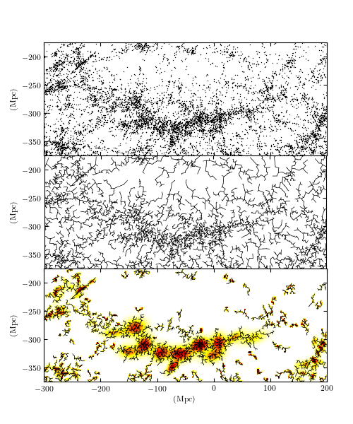
An approximate Euclidean minimum spanning tree over the two-dimensional projection of the SDSS Great Wall. The upper panel shows the input points, and the middle panel shows the dendrogram connecting them. The lower panel shows clustering based on this dendrogram, created by removing the largest 10% of the graph edges, and keeping the remaining connected clusters with 30 or more members.

Additional information

This figure is based on the data presented in Figure 1 of Cowan & Ivezic (2008). A similar figure appears in the book “Statistics, Data Mining, and Machine Learning in Astronomy”, by Ivezic, Connolly, Vanderplas, and Gray (2013).

The three panels of this figure show a hierarchical clustering of a subset of galaxies from the Sloan Digital Sky Survey (SDSS). This region is known as the “SDSS Great Wall”, and contains an extended cluster of several thousand galaxies approximately 300Mpc (about 1 billion light years) from earth. The top panel shows the positions of over 8,000 galaxies projected to a 2D plane with Earth at the point (0, 0). The middle panel shows a dendrogram representation of a Euclidean Minimum Spanning Tree (MST) over the galaxy locations. By eliminating edges of a MST which are greater than a given length, we can measure the amount of clustering at that scale: this is one version of a class of models known as Hierarchical Clustering. The bottom panel shows the results of this clustering approach for an edge cutoff of 3.5Mpc, along with a Gaussian Mixture Model fit to the distribution within each cluster.

Code output:

 scale: 3.54953 Mpc

Python source code:

# Author: Jake VanderPlas
# License: BSD
#   The figure produced by this code is published in the textbook
#   "Statistics, Data Mining, and Machine Learning in Astronomy" (2013)
#   For more information, see http://astroML.github.com
#   To report a bug or issue, use the following forum:
#    https://groups.google.com/forum/#!forum/astroml-general

from __future__ import print_function, division

import numpy as np
from matplotlib import pyplot as plt

from scipy import sparse
from sklearn.mixture import GaussianMixture

from astroML.clustering import HierarchicalClustering, get_graph_segments
from astroML.datasets import fetch_great_wall

#----------------------------------------------------------------------
# This function adjusts matplotlib settings for a uniform feel in the textbook.
# Note that with usetex=True, fonts are rendered with LaTeX.  This may
# result in an error if LaTeX is not installed on your system.  In that case,
# you can set usetex to False.
if "setup_text_plots" not in globals():
    from astroML.plotting import setup_text_plots
setup_text_plots(fontsize=8, usetex=True)

#------------------------------------------------------------
# get data
X = fetch_great_wall()

xmin, xmax = (-375, -175)
ymin, ymax = (-300, 200)

#------------------------------------------------------------
# Compute the MST clustering model
n_neighbors = 10
edge_cutoff = 0.9
cluster_cutoff = 10
model = HierarchicalClustering(n_neighbors=10,
                               edge_cutoff=edge_cutoff,
                               min_cluster_size=cluster_cutoff)
model.fit(X)
print(" scale: %2g Mpc" % np.percentile(model.full_tree_.data,
                                        100 * edge_cutoff))

n_components = model.n_components_
labels = model.labels_

#------------------------------------------------------------
# Get the x, y coordinates of the beginning and end of each line segment
T_x, T_y = get_graph_segments(model.X_train_,
                              model.full_tree_)
T_trunc_x, T_trunc_y = get_graph_segments(model.X_train_,
                                          model.cluster_graph_)

#------------------------------------------------------------
# Fit a GaussianMixture to each individual cluster
Nx = 100
Ny = 250
Xgrid = np.vstack(map(np.ravel, np.meshgrid(np.linspace(xmin, xmax, Nx),
                                            np.linspace(ymin, ymax, Ny)))).T
density = np.zeros(Xgrid.shape[0])

for i in range(n_components):
    ind = (labels == i)
    Npts = ind.sum()
    Nclusters = min(12, Npts // 5)
    gmm = GaussianMixture(Nclusters, random_state=0).fit(X[ind])
    dens = np.exp(gmm.score_samples(Xgrid))
    density += dens / dens.max()

density = density.reshape((Ny, Nx))

#----------------------------------------------------------------------
# Plot the results
fig = plt.figure(figsize=(5, 6))
fig.subplots_adjust(hspace=0, left=0.1, right=0.95, bottom=0.1, top=0.9)

ax = fig.add_subplot(311, aspect='equal')
ax.scatter(X[:, 1], X[:, 0], s=1, lw=0, c='k')
ax.set_xlim(ymin, ymax)
ax.set_ylim(xmin, xmax)
ax.xaxis.set_major_formatter(plt.NullFormatter())
ax.set_ylabel('(Mpc)')

ax = fig.add_subplot(312, aspect='equal')
ax.plot(T_y, T_x, c='k', lw=0.5)
ax.set_xlim(ymin, ymax)
ax.set_ylim(xmin, xmax)
ax.xaxis.set_major_formatter(plt.NullFormatter())
ax.set_ylabel('(Mpc)')

ax = fig.add_subplot(313, aspect='equal')
ax.plot(T_trunc_y, T_trunc_x, c='k', lw=0.5)
ax.imshow(density.T, origin='lower', cmap=plt.cm.hot_r,
          extent=[ymin, ymax, xmin, xmax])

ax.set_xlim(ymin, ymax)
ax.set_ylim(xmin, xmax)
ax.set_xlabel('(Mpc)')
ax.set_ylabel('(Mpc)')

plt.show()

[download source: fig_great_wall_MST.py]