Mean Shift Example

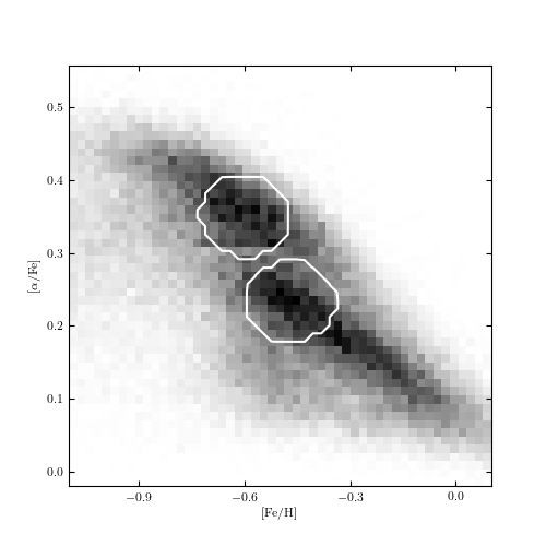
Figure 6.14

Mean-shift clustering on the metallicity datas et used in figures 6.6 and 6.13. The method finds two clusters associated with local maxima of the distribution (interior of the circles). Points outside the circles have been determined to lie in the background. The mean shift does not attempt to model correlation in the clusters: that is, the resulting clusters are axis aligned.

Code output:

[-1  0  1]
0.4
number of estimated clusters : 2

Python source code:

# Author: Jake VanderPlas
# License: BSD
#   The figure produced by this code is published in the textbook
#   "Statistics, Data Mining, and Machine Learning in Astronomy" (2013)
#   For more information, see http://astroML.github.com
#   To report a bug or issue, use the following forum:
#    https://groups.google.com/forum/#!forum/astroml-general

from __future__ import print_function

import numpy as np
from matplotlib import pyplot as plt
from matplotlib.patches import Ellipse
from scipy.stats import norm

from sklearn.cluster import MeanShift, estimate_bandwidth
from sklearn import preprocessing

from astroML.datasets import fetch_sdss_sspp

#----------------------------------------------------------------------
# This function adjusts matplotlib settings for a uniform feel in the textbook.
# Note that with usetex=True, fonts are rendered with LaTeX.  This may
# result in an error if LaTeX is not installed on your system.  In that case,
# you can set usetex to False.
if "setup_text_plots" not in globals():
    from astroML.plotting import setup_text_plots
setup_text_plots(fontsize=8, usetex=True)

#------------------------------------------------------------
# Get the data
np.random.seed(0)
data = fetch_sdss_sspp(cleaned=True)

# cut out some additional strange outliers
data = data[~((data['alphFe'] > 0.4) & (data['FeH'] > -0.3))]

X = np.vstack([data['FeH'], data['alphFe']]).T

#----------------------------------------------------------------------
# Compute clustering with MeanShift
#
# We'll work with the scaled data, because MeanShift finds circular clusters

X_scaled = preprocessing.scale(X)

# The following bandwidth can be automatically detected using
# the routine estimate_bandwidth().  Because bandwidth estimation
# is very expensive in memory and computation, we'll skip it here.

#bandwidth = estimate_bandwidth(X)
bandwidth = 0.4

ms = MeanShift(bandwidth=bandwidth, bin_seeding=True, cluster_all=False)
ms.fit(X_scaled)

labels_unique = np.unique(ms.labels_)
n_clusters = len(labels_unique[labels_unique >= 0])
print(labels_unique)
print(bandwidth)
print("number of estimated clusters :", n_clusters)

#------------------------------------------------------------
# Plot the results
fig = plt.figure(figsize=(5, 5))
ax = fig.add_subplot(111)

# plot density
H, FeH_bins, alphFe_bins = np.histogram2d(data['FeH'], data['alphFe'], 51)

ax.imshow(H.T, origin='lower', interpolation='nearest', aspect='auto',
          extent=[FeH_bins[0], FeH_bins[-1],
                  alphFe_bins[0], alphFe_bins[-1]],
          cmap=plt.cm.binary)

# plot clusters
colors = ['b', 'g', 'r', 'k']

for i in range(n_clusters):
    Xi = X[ms.labels_ == i]
    H, b1, b2 = np.histogram2d(Xi[:, 0], Xi[:, 1], (FeH_bins, alphFe_bins))

    bins = [0.1]

    ax.contour(0.5 * (FeH_bins[1:] + FeH_bins[:-1]),
               0.5 * (alphFe_bins[1:] + alphFe_bins[:-1]),
               H.T, bins, colors='w')

ax.xaxis.set_major_locator(plt.MultipleLocator(0.3))
ax.set_xlim(-1.101, 0.101)
ax.set_ylim(alphFe_bins[0], alphFe_bins[-1])
ax.set_xlabel(r'$\rm [Fe/H]$')
ax.set_ylabel(r'$\rm [\alpha/Fe]$')

plt.show()

[download source: fig_meanshift_metallicity.py]