Example of Fisher’s F distribution

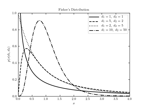
Figure 3.16.

This shows an example of Fisher’s F distribution with various parameters. We’ll generate the distribution using:

dist = scipy.stats.f(...)

Where … should be filled in with the desired distribution parameters Once we have defined the distribution parameters in this way, these distribution objects have many useful methods; for example:

• dist.pmf(x) computes the Probability Mass Function at values x in the case of discrete distributions

• dist.pdf(x) computes the Probability Density Function at values x in the case of continuous distributions

• dist.rvs(N) computes N random variables distributed according to the given distribution

Many further options exist; refer to the documentation of scipy.stats for more details.

Code output:

Python source code:

# Author: Jake VanderPlas
# License: BSD
#   The figure produced by this code is published in the textbook
#   "Statistics, Data Mining, and Machine Learning in Astronomy" (2013)
#   For more information, see http://astroML.github.com
#   To report a bug or issue, use the following forum:
#    https://groups.google.com/forum/#!forum/astroml-general
import numpy as np
from scipy.stats import f as fisher_f
from matplotlib import pyplot as plt

#----------------------------------------------------------------------
# This function adjusts matplotlib settings for a uniform feel in the textbook.
# Note that with usetex=True, fonts are rendered with LaTeX.  This may
# result in an error if LaTeX is not installed on your system.  In that case,
# you can set usetex to False.
if "setup_text_plots" not in globals():
    from astroML.plotting import setup_text_plots
setup_text_plots(fontsize=8, usetex=True)

#------------------------------------------------------------
# Define the distribution parameters to be plotted
mu = 0
d1_values = [1, 5, 2, 10]
d2_values = [1, 2, 5, 50]
linestyles = ['-', '--', ':', '-.']
x = np.linspace(0, 5, 1001)[1:]

fig, ax = plt.subplots(figsize=(5, 3.75))

for (d1, d2, ls) in zip(d1_values, d2_values, linestyles):
    dist = fisher_f(d1, d2, mu)

    plt.plot(x, dist.pdf(x), ls=ls, c='black',
             label=r'$d_1=%i,\ d_2=%i$' % (d1, d2))

plt.xlim(0, 4)
plt.ylim(0.0, 1.0)

plt.xlabel('$x$')
plt.ylabel(r'$p(x|d_1, d_2)$')
plt.title("Fisher's Distribution")

plt.legend()
plt.show()

[download source: fig_fisher_f_distribution.py]