Example of a Fourier Transform

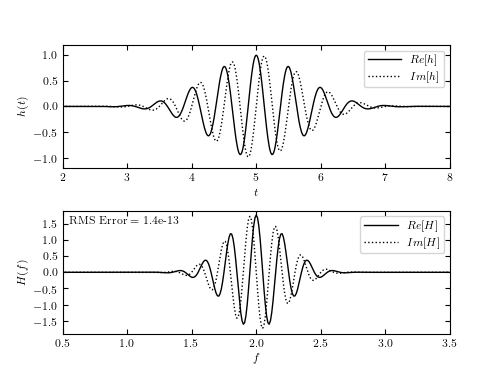
Figure E.1

An example of approximating the continuous Fourier transform of a function using the fast Fourier transform.

Code output:

Python source code:

# Author: Jake VanderPlas
# License: BSD
#   The figure produced by this code is published in the textbook
#   "Statistics, Data Mining, and Machine Learning in Astronomy" (2013)
#   For more information, see http://astroML.github.com
#   To report a bug or issue, use the following forum:
#    https://groups.google.com/forum/#!forum/astroml-general
import numpy as np
from matplotlib import pyplot as plt
from scipy import fftpack

from astroML.fourier import FT_continuous, sinegauss, sinegauss_FT

#----------------------------------------------------------------------
# This function adjusts matplotlib settings for a uniform feel in the textbook.
# Note that with usetex=True, fonts are rendered with LaTeX.  This may
# result in an error if LaTeX is not installed on your system.  In that case,
# you can set usetex to False.
if "setup_text_plots" not in globals():
    from astroML.plotting import setup_text_plots
setup_text_plots(fontsize=8, usetex=True)

#------------------------------------------------------------
# Choose parameters for the wavelet
N = 10000
t0 = 5
f0 = 2
Q = 2

#------------------------------------------------------------
# Compute the wavelet on a grid of times
Dt = 0.01
t = t0 + Dt * (np.arange(N) - N / 2)
h = sinegauss(t, t0, f0, Q)

#------------------------------------------------------------
# Approximate the continuous Fourier Transform
f, H = FT_continuous(t, h)

rms_err = np.sqrt(np.mean(abs(H - sinegauss_FT(f, t0, f0, Q)) ** 2))

#------------------------------------------------------------
# Plot the results
fig = plt.figure(figsize=(5, 3.75))
fig.subplots_adjust(hspace=0.35)

# plot the wavelet
ax = fig.add_subplot(211)
ax.plot(t, h.real, '-', c='black', label='$Re[h]$', lw=1)
ax.plot(t, h.imag, ':', c='black', label='$Im[h]$', lw=1)
ax.legend()

ax.set_xlim(2, 8)
ax.set_ylim(-1.2, 1.2)
ax.set_xlabel('$t$')
ax.set_ylabel('$h(t)$')

# plot the Fourier transform
ax = fig.add_subplot(212)
ax.plot(f, H.real, '-', c='black', label='$Re[H]$', lw=1)
ax.plot(f, H.imag, ':', c='black', label='$Im[H]$', lw=1)
ax.text(0.55, 1.5, "RMS Error = %.2g" % rms_err)
ax.legend()

ax.set_xlim(0.5, 3.5)
ax.set_ylim(-1.9, 1.9)
ax.set_xlabel('$f$')
ax.set_ylabel('$H(f)$')

plt.show()

[download source: fig_fft_text_example.py]