Multiband Lomb-Scargle Periodogram

Though classical periodogram approaches only handle a single band of data, multiband extensions have been recently proposed. gatspy implements one which was suggested by VanderPlas et al. The interface is almost identical to that discussed in Lomb-Scargle Periodogram, with the exception of the fit() method and predict() method requiring a specification of the filters.

Two versions of the multiband periodogram are available:

LombScargleMultiband

This class implements the flexible multiband model described in VanderPlas (2015). In particular, it uses regularization to push common variation into a base model, which effectively simplifies the overall model and leads to less background signal in the periodogram.

LombScargleMultibandFast

This class is a faster version of the multiband periodogram without regularization. This means that it cannot fit the same range of models as LombScargleMultiband, but essentially just combines several independent band-by-band fits.

Here is a quick example of finding the best period in multiband data. We’ll use LombScargleMultibandFast here. We start by loading the lightcurve (for more information, see Datasets (gatspy.datasets)):

In [1]: from gatspy import datasets, periodic

In [2]: rrlyrae = datasets.fetch_rrlyrae()

In [3]: lcid = rrlyrae.ids[0]

In [4]: t, mag, dmag, filts = rrlyrae.get_lightcurve(lcid)

With this lightcurve specified, we can now build and fit the model:

In [5]: model = periodic.LombScargleMultibandFast(fit_period=True)

In [6]: model.optimizer.period_range=(0.5, 0.7)

In [7]: model.fit(t, mag, dmag, filts);

And, as with the single-band version, the best period is now stored as an attribute of the model:

In [8]: model.best_period
Out[8]: 0.61431670719850195

Once the model is fit, we can then use the predict() method to look at the model prediction for any given band:

In [9]: tfit = np.linspace(0, model.best_period, 1000)

In [10]: magfit = model.predict(tfit, filts='g')

In [11]: magfit[:4]
Out[11]: array([ 17.1411512 ,  17.13947457,  17.13780707,  17.13614876])

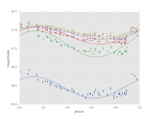
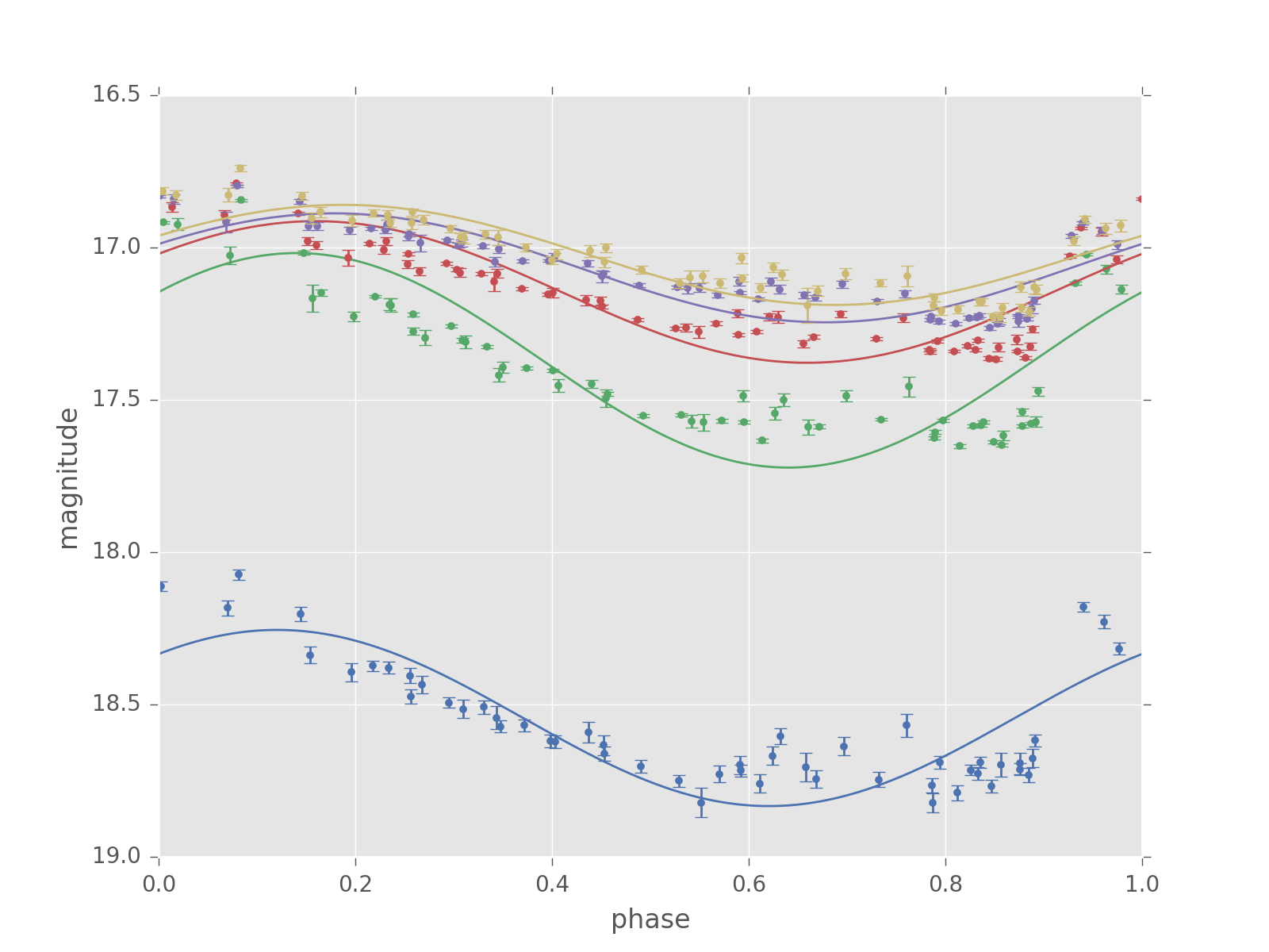
Below is a plot of the magnitudes at this best-fit period:

(Source code, png, hires.png, pdf)

We see that the simplest multiband model is just a set of offset sine fits to the individual bands. As in the single-band case, the model is not a particularly good fit to the data, but nevertheless it is useful in determining the period from the data.

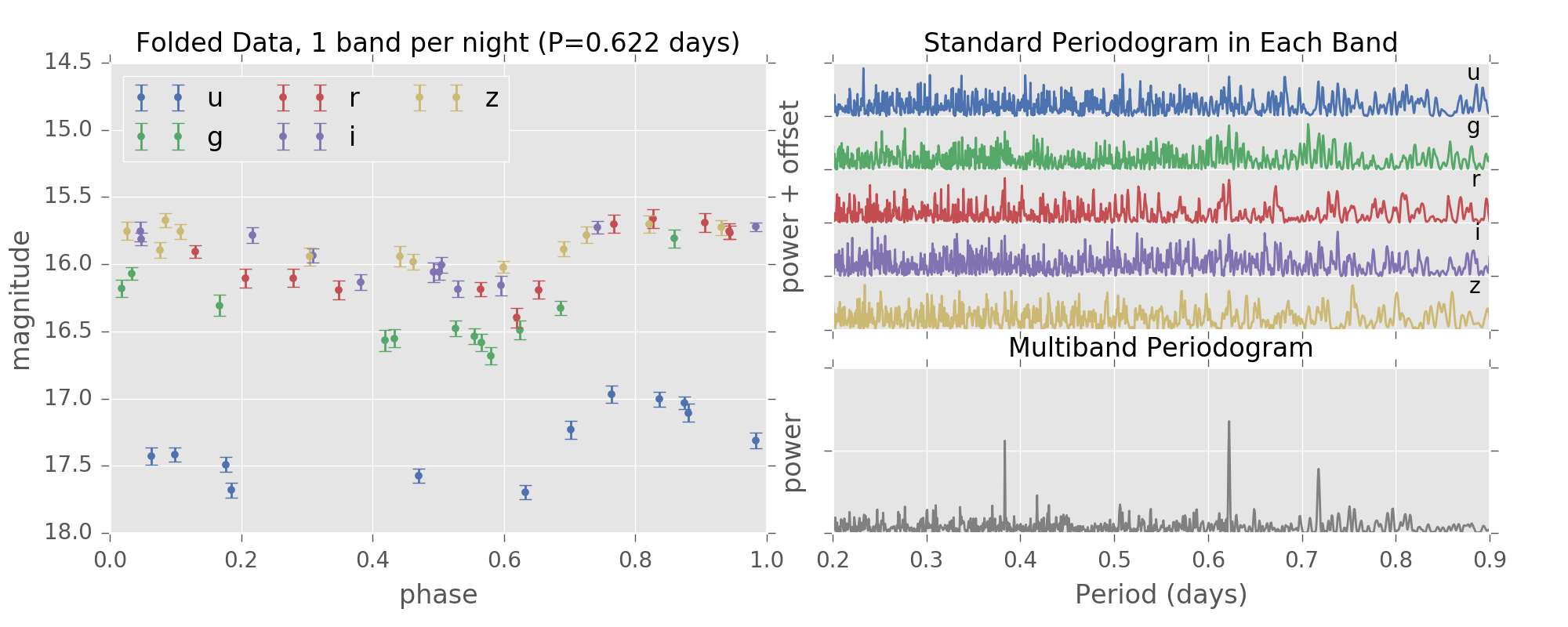
A more sophisticated multiband approach involves model simplification via a regularization term that pushes common variation into a “base model”; this is slightly slower to compute, but can be accomplished with the LombScargleMultiband model. For example, here is a comparison of the single-band periodograms to this regularized multiband model on six months of sparsely-sampled LSST-style data:

(Source code, png, hires.png, pdf)

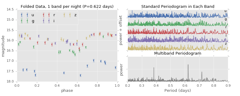
Notice in this figure that periodograms built from individual bands fail to locate the frequency, while the periodogram built from the entire dataset has a strong spike in power at the correct frequency.

For more information on these multiband methods, see the VanderPlas et al. paper, and the associated figure code at http://github.com/jakevdp/multiband_LS/