Gaussian Naive Bayes Classification of photometry

Figure 9.3

Gaussian naive Bayes classification method used to separate variable RR Lyrae stars from nonvariable main sequence stars. In the left panel, the light gray points show non- variable sources, while the dark points show variable sources. The classification boundary is shown by the black line, and the classification probability is shown by the shaded background. In the right panel, we show the completeness and contamination as a function of the number of features used in the fit. For the single feature, u - g is used. For two features, u - g and g = r areused. For three features, u - g, g - r, and r- i are used. It is evident that the g - r color is the best discriminator. With all four colors, naive Bayes attains a completeness of 0.876 and a contamination of 0.790.

Code output:

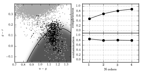
completeness [ 0.48175182  0.68613139  0.81021898  0.87591241]
contamination [ 0.85201794  0.79295154  0.80143113  0.79020979]

Python source code:

# Author: Jake VanderPlas
# License: BSD
#   The figure produced by this code is published in the textbook
#   "Statistics, Data Mining, and Machine Learning in Astronomy" (2013)
#   For more information, see http://astroML.github.com
#   To report a bug or issue, use the following forum:
#    https://groups.google.com/forum/#!forum/astroml-general
import numpy as np
from matplotlib import pyplot as plt

from sklearn.naive_bayes import GaussianNB
from astroML.datasets import fetch_rrlyrae_combined
from astroML.utils import split_samples
from astroML.utils import completeness_contamination

#----------------------------------------------------------------------
# This function adjusts matplotlib settings for a uniform feel in the textbook.
# Note that with usetex=True, fonts are rendered with LaTeX.  This may
# result in an error if LaTeX is not installed on your system.  In that case,
# you can set usetex to False.
from astroML.plotting import setup_text_plots
setup_text_plots(fontsize=8, usetex=True)

#----------------------------------------------------------------------
# get data and split into training & testing sets
X, y = fetch_rrlyrae_combined()
X = X[:, [1, 0, 2, 3]]  # rearrange columns for better 1-color results
(X_train, X_test), (y_train, y_test) = split_samples(X, y, [0.75, 0.25],
                                                     random_state=0)

N_tot = len(y)
N_st = np.sum(y == 0)
N_rr = N_tot - N_st
N_train = len(y_train)
N_test = len(y_test)
N_plot = 5000 + N_rr

#----------------------------------------------------------------------
# perform Naive Bayes
classifiers = []
predictions = []
Ncolors = np.arange(1, X.shape[1] + 1)

order = np.array([1, 0, 2, 3])

for nc in Ncolors:
    clf = GaussianNB()
    clf.fit(X_train[:, :nc], y_train)
    y_pred = clf.predict(X_test[:, :nc])

    classifiers.append(clf)
    predictions.append(y_pred)

completeness, contamination = completeness_contamination(predictions, y_test)

print "completeness", completeness
print "contamination", contamination

#------------------------------------------------------------
# Compute the decision boundary
clf = classifiers[1]
xlim = (0.7, 1.35)
ylim = (-0.15, 0.4)

xx, yy = np.meshgrid(np.linspace(xlim[0], xlim[1], 81),
                     np.linspace(ylim[0], ylim[1], 71))

Z = clf.predict_proba(np.c_[yy.ravel(), xx.ravel()])
Z = Z[:, 1].reshape(xx.shape)

#----------------------------------------------------------------------
# plot the results
fig = plt.figure(figsize=(5, 2.5))
fig.subplots_adjust(bottom=0.15, top=0.95, hspace=0.0,
                    left=0.1, right=0.95, wspace=0.2)

# left plot: data and decision boundary
ax = fig.add_subplot(121)
im = ax.scatter(X[-N_plot:, 1], X[-N_plot:, 0], c=y[-N_plot:],
                s=4, lw=0, cmap=plt.cm.binary, zorder=2)
im.set_clim(-0.5, 1)

im = ax.imshow(Z, origin='lower', aspect='auto',
               cmap=plt.cm.binary, zorder=1,
               extent=xlim + ylim)
im.set_clim(0, 1.5)
ax.contour(xx, yy, Z, [0.5], colors='k')

ax.set_xlim(xlim)
ax.set_ylim(ylim)

ax.set_xlabel('$u-g$')
ax.set_ylabel('$g-r$')

# Plot completeness vs Ncolors
ax = plt.subplot(222)
ax.plot(Ncolors, completeness, 'o-k', ms=6)

ax.xaxis.set_major_locator(plt.MultipleLocator(1))
ax.yaxis.set_major_locator(plt.MultipleLocator(0.2))
ax.xaxis.set_major_formatter(plt.NullFormatter())

ax.set_ylabel('completeness')
ax.set_xlim(0.5, 4.5)
ax.set_ylim(-0.1, 1.1)
ax.grid(True)

# Plot contamination vs Ncolors
ax = plt.subplot(224)
ax.plot(Ncolors, contamination, 'o-k', ms=6)

ax.xaxis.set_major_locator(plt.MultipleLocator(1))
ax.yaxis.set_major_locator(plt.MultipleLocator(0.2))
ax.xaxis.set_major_formatter(plt.FormatStrFormatter('%i'))

ax.set_xlabel('N colors')
ax.set_ylabel('contamination')
ax.set_xlim(0.5, 4.5)
ax.set_ylim(-0.1, 1.1)
ax.grid(True)

plt.show()

[download source: fig_rrlyrae_naivebayes.py]