Decision Tree Classification of photometry

Figure 9.13

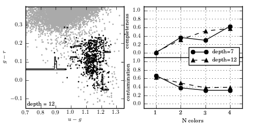
Decision tree applied to the RR Lyrae data (see caption of figure 9.3 for details). This example uses tree depths of 7 and 12. With all four colors,this decision tree achieves a completeness of 0.569 and a contamination of 0.386.

Code output:

completeness [[ 0.00729927  0.3649635   0.29927007  0.62773723]
 [ 0.02189781  0.31386861  0.51824818  0.57664234]]
contamination [[ 0.66666667  0.375       0.31666667  0.31746032]
 [ 0.625       0.48809524  0.37719298  0.3875969 ]]

Python source code:

# Author: Jake VanderPlas
# License: BSD
#   The figure produced by this code is published in the textbook
#   "Statistics, Data Mining, and Machine Learning in Astronomy" (2013)
#   For more information, see http://astroML.github.com
#   To report a bug or issue, use the following forum:
#    https://groups.google.com/forum/#!forum/astroml-general
import numpy as np
from matplotlib import pyplot as plt

from sklearn.tree import DecisionTreeClassifier
from astroML.datasets import fetch_rrlyrae_combined
from astroML.utils import split_samples
from astroML.utils import completeness_contamination

#----------------------------------------------------------------------
# This function adjusts matplotlib settings for a uniform feel in the textbook.
# Note that with usetex=True, fonts are rendered with LaTeX.  This may
# result in an error if LaTeX is not installed on your system.  In that case,
# you can set usetex to False.
from astroML.plotting import setup_text_plots
setup_text_plots(fontsize=8, usetex=True)

#----------------------------------------------------------------------
# get data and split into training & testing sets
X, y = fetch_rrlyrae_combined()
X = X[:, [1, 0, 2, 3]]  # rearrange columns for better 1-color results
(X_train, X_test), (y_train, y_test) = split_samples(X, y, [0.75, 0.25],
                                                     random_state=0)
N_tot = len(y)
N_st = np.sum(y == 0)
N_rr = N_tot - N_st
N_train = len(y_train)
N_test = len(y_test)
N_plot = 5000 + N_rr

#----------------------------------------------------------------------
# Fit Decision tree
Ncolors = np.arange(1, X.shape[1] + 1)

classifiers = []
predictions = []
Ncolors = np.arange(1, X.shape[1] + 1)
depths = [7, 12]

for depth in depths:
    classifiers.append([])
    predictions.append([])
    for nc in Ncolors:
        clf = DecisionTreeClassifier(random_state=0, max_depth=depth,
                                     criterion='entropy')
        clf.fit(X_train[:, :nc], y_train)
        y_pred = clf.predict(X_test[:, :nc])

        classifiers[-1].append(clf)
        predictions[-1].append(y_pred)

completeness, contamination = completeness_contamination(predictions, y_test)

print "completeness", completeness
print "contamination", contamination

#------------------------------------------------------------
# compute the decision boundary

clf = classifiers[1][1]
xlim = (0.7, 1.35)
ylim = (-0.15, 0.4)

xx, yy = np.meshgrid(np.linspace(xlim[0], xlim[1], 101),
                     np.linspace(ylim[0], ylim[1], 101))

Z = clf.predict(np.c_[yy.ravel(), xx.ravel()])
Z = Z.reshape(xx.shape)

#----------------------------------------------------------------------
# plot the results
fig = plt.figure(figsize=(5, 2.5))
fig.subplots_adjust(bottom=0.15, top=0.95, hspace=0.0,
                    left=0.1, right=0.95, wspace=0.2)

# left plot: data and decision boundary
ax = fig.add_subplot(121)
im = ax.scatter(X[-N_plot:, 1], X[-N_plot:, 0], c=y[-N_plot:],
                s=4, lw=0, cmap=plt.cm.binary, zorder=2)
im.set_clim(-0.5, 1)

ax.contour(xx, yy, Z, [0.5], colors='k')

ax.set_xlim(xlim)
ax.set_ylim(ylim)

ax.set_xlabel('$u-g$')
ax.set_ylabel('$g-r$')

ax.text(0.02, 0.02, "depth = %i" % depths[1],
        transform=ax.transAxes)

# plot completeness vs Ncolors
ax = fig.add_subplot(222)
ax.plot(Ncolors, completeness[0], 'o-k', ms=6, label="depth=%i" % depths[0])
ax.plot(Ncolors, completeness[1], '^--k', ms=6, label="depth=%i" % depths[1])

ax.xaxis.set_major_locator(plt.MultipleLocator(1))
ax.yaxis.set_major_locator(plt.MultipleLocator(0.2))
ax.xaxis.set_major_formatter(plt.NullFormatter())

ax.set_ylabel('completeness')
ax.set_xlim(0.5, 4.5)
ax.set_ylim(-0.1, 1.1)
ax.grid(True)

# plot contamination vs Ncolors
ax = fig.add_subplot(224)
ax.plot(Ncolors, contamination[0], 'o-k', ms=6, label="depth=%i" % depths[0])
ax.plot(Ncolors, contamination[1], '^--k', ms=6, label="depth=%i" % depths[1])
ax.legend(loc='lower right',
          bbox_to_anchor=(1.0, 0.79))

ax.xaxis.set_major_locator(plt.MultipleLocator(1))
ax.yaxis.set_major_locator(plt.MultipleLocator(0.2))
ax.xaxis.set_major_formatter(plt.FormatStrFormatter('%i'))

ax.set_xlabel('N colors')
ax.set_ylabel('contamination')
ax.set_xlim(0.5, 4.5)
ax.set_ylim(-0.1, 1.1)
ax.grid(True)

plt.show()

[download source: fig_rrlyrae_decisiontree.py]