Perform Outlier Rejection with MCMC
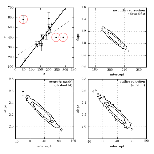
Figure 8.9
Bayesian outlier detection for the same data as shown in figure 8.8. The top-left panel shows the data, with the fits from each model. The top-right panel shows the 1-sigma and 2-sigma contours for the slope and intercept with no outlier correction: the resulting fit (shown by the dotted line) is clearly highly affected by the presence of outliers. The bottom-left panel shows the marginalized 1-sigma and 2-sigma contours for a mixture model (eq. 8.67). The bottom-right panel shows the marginalized 1-sigma and 2-sigma contours for a model in which points are identified individually as “good” or “bad” (eq. 8.68). The points which are identified by this method as bad with a probability greater than 68% are circled in the first panel.
[--------         21%                  ] 5291 of 25000 complete in 0.5 sec
[--------------   37%                  ] 9363 of 25000 complete in 1.0 sec
[-----------------54%                  ] 13636 of 25000 complete in 1.5 sec
[-----------------71%-------           ] 17823 of 25000 complete in 2.0 sec
[-----------------88%-------------     ] 22063 of 25000 complete in 2.5 sec
[-----------------100%-----------------] 25000 of 25000 complete in 2.9 sec
[-                 2%                  ] 697 of 25000 complete in 0.5 sec
[--                5%                  ] 1366 of 25000 complete in 1.0 sec
[---               8%                  ] 2030 of 25000 complete in 1.5 sec
[----             10%                  ] 2682 of 25000 complete in 2.0 sec
[-----            13%                  ] 3350 of 25000 complete in 2.5 sec
[------           16%                  ] 4013 of 25000 complete in 3.0 sec
[-------          18%                  ] 4669 of 25000 complete in 3.5 sec
[--------         21%                  ] 5300 of 25000 complete in 4.0 sec
[--------         23%                  ] 5907 of 25000 complete in 4.5 sec
[---------        26%                  ] 6511 of 25000 complete in 5.0 sec
[----------       28%                  ] 7130 of 25000 complete in 5.5 sec
[-----------      30%                  ] 7740 of 25000 complete in 6.0 sec
[------------     33%                  ] 8365 of 25000 complete in 6.5 sec
[-------------    35%                  ] 8972 of 25000 complete in 7.0 sec
[--------------   38%                  ] 9581 of 25000 complete in 7.5 sec
[---------------  40%                  ] 10206 of 25000 complete in 8.0 sec
[---------------- 43%                  ] 10814 of 25000 complete in 8.5 sec
[-----------------45%                  ] 11428 of 25000 complete in 9.0 sec
[-----------------48%                  ] 12056 of 25000 complete in 9.5 sec
[-----------------50%                  ] 12679 of 25000 complete in 10.0 sec
[-----------------53%                  ] 13310 of 25000 complete in 10.5 sec
[-----------------55%-                 ] 13930 of 25000 complete in 11.0 sec
[-----------------58%--                ] 14564 of 25000 complete in 11.5 sec
[-----------------60%---               ] 15182 of 25000 complete in 12.0 sec
[-----------------63%----              ] 15806 of 25000 complete in 12.5 sec
[-----------------65%----              ] 16429 of 25000 complete in 13.0 sec
[-----------------68%-----             ] 17062 of 25000 complete in 13.5 sec
[-----------------70%------            ] 17686 of 25000 complete in 14.0 sec
[-----------------73%-------           ] 18289 of 25000 complete in 14.5 sec
[-----------------75%--------          ] 18905 of 25000 complete in 15.0 sec
[-----------------78%---------         ] 19511 of 25000 complete in 15.5 sec
[-----------------80%----------        ] 20136 of 25000 complete in 16.0 sec
[-----------------82%-----------       ] 20745 of 25000 complete in 16.5 sec
[-----------------85%------------      ] 21343 of 25000 complete in 17.0 sec
[-----------------87%-------------     ] 21949 of 25000 complete in 17.5 sec
[-----------------90%--------------    ] 22559 of 25000 complete in 18.0 sec
[-----------------92%---------------   ] 23169 of 25000 complete in 18.5 sec
[-----------------95%----------------  ] 23766 of 25000 complete in 19.0 sec
[-----------------97%----------------- ] 24379 of 25000 complete in 19.5 sec
[-----------------99%----------------- ] 24993 of 25000 complete in 20.0 sec
[-----------------100%-----------------] 25000 of 25000 complete in 20.0 sec
[                  2%                  ] 558 of 25000 complete in 0.5 sec
[-                 4%                  ] 1099 of 25000 complete in 1.0 sec
[--                6%                  ] 1641 of 25000 complete in 1.5 sec
[---               8%                  ] 2165 of 25000 complete in 2.0 sec
[----             10%                  ] 2702 of 25000 complete in 2.5 sec
[----             12%                  ] 3230 of 25000 complete in 3.0 sec
[-----            14%                  ] 3740 of 25000 complete in 3.5 sec
[------           17%                  ] 4266 of 25000 complete in 4.0 sec
[-------          19%                  ] 4789 of 25000 complete in 4.5 sec
[--------         21%                  ] 5278 of 25000 complete in 5.0 sec
[--------         23%                  ] 5756 of 25000 complete in 5.5 sec
[---------        25%                  ] 6259 of 25000 complete in 6.0 sec
[----------       27%                  ] 6766 of 25000 complete in 6.5 sec
[-----------      28%                  ] 7242 of 25000 complete in 7.0 sec
[-----------      30%                  ] 7747 of 25000 complete in 7.5 sec
[------------     33%                  ] 8253 of 25000 complete in 8.0 sec
[-------------    35%                  ] 8758 of 25000 complete in 8.5 sec
[--------------   37%                  ] 9258 of 25000 complete in 9.0 sec
[--------------   39%                  ] 9757 of 25000 complete in 9.5 sec
[---------------  41%                  ] 10258 of 25000 complete in 10.0 sec
[---------------- 43%                  ] 10765 of 25000 complete in 10.5 sec
[-----------------45%                  ] 11264 of 25000 complete in 11.0 sec
[-----------------47%                  ] 11768 of 25000 complete in 11.5 sec
[-----------------49%                  ] 12260 of 25000 complete in 12.0 sec
[-----------------51%                  ] 12761 of 25000 complete in 12.5 sec
[-----------------53%                  ] 13262 of 25000 complete in 13.0 sec
[-----------------55%                  ] 13773 of 25000 complete in 13.5 sec
[-----------------57%-                 ] 14275 of 25000 complete in 14.0 sec
[-----------------59%--                ] 14757 of 25000 complete in 14.5 sec
[-----------------60%---               ] 15244 of 25000 complete in 15.0 sec
[-----------------62%---               ] 15748 of 25000 complete in 15.5 sec
[-----------------64%----              ] 16240 of 25000 complete in 16.0 sec
[-----------------66%-----             ] 16743 of 25000 complete in 16.5 sec
[-----------------68%------            ] 17235 of 25000 complete in 17.0 sec
[-----------------70%------            ] 17729 of 25000 complete in 17.5 sec
[-----------------72%-------           ] 18214 of 25000 complete in 18.0 sec
[-----------------74%--------          ] 18710 of 25000 complete in 18.5 sec
[-----------------76%---------         ] 19197 of 25000 complete in 19.0 sec
[-----------------78%---------         ] 19695 of 25000 complete in 19.5 sec
[-----------------80%----------        ] 20189 of 25000 complete in 20.0 sec
[-----------------82%-----------       ] 20685 of 25000 complete in 20.5 sec
[-----------------84%------------      ] 21174 of 25000 complete in 21.0 sec
[-----------------86%------------      ] 21665 of 25000 complete in 21.5 sec
[-----------------88%-------------     ] 22144 of 25000 complete in 22.0 sec
[-----------------90%--------------    ] 22642 of 25000 complete in 22.5 sec
[-----------------92%---------------   ] 23145 of 25000 complete in 23.0 sec
[-----------------94%---------------   ] 23653 of 25000 complete in 23.5 sec
[-----------------96%----------------  ] 24159 of 25000 complete in 24.0 sec
[-----------------98%----------------- ] 24657 of 25000 complete in 24.5 sec
[-----------------100%-----------------] 25000 of 25000 complete in 24.9 sec
# Author: Jake VanderPlas
# License: BSD
#   The figure produced by this code is published in the textbook
#   "Statistics, Data Mining, and Machine Learning in Astronomy" (2013)
#   For more information, see http://astroML.github.com
#   To report a bug or issue, use the following forum:
#    https://groups.google.com/forum/#!forum/astroml-general
import numpy as np
from matplotlib import pyplot as plt
from astroML.datasets import fetch_hogg2010test
from astroML.plotting.mcmc import convert_to_stdev

# Hack to fix import issue in older versions of pymc
import scipy
import scipy.misc
scipy.derivative = scipy.misc.derivative
import pymc

#----------------------------------------------------------------------
# This function adjusts matplotlib settings for a uniform feel in the textbook.
# Note that with usetex=True, fonts are rendered with LaTeX.  This may
# result in an error if LaTeX is not installed on your system.  In that case,
# you can set usetex to False.
from astroML.plotting import setup_text_plots
setup_text_plots(fontsize=8, usetex=True)

np.random.seed(0)

#------------------------------------------------------------
# Get data: this includes outliers
data = fetch_hogg2010test()
xi = data['x']
yi = data['y']
dyi = data['sigma_y']


#----------------------------------------------------------------------
# First model: no outlier correction
# define priors on beta = (slope, intercept)
@pymc.stochastic
def beta_M0(value=np.array([2., 100.])):
    """Slope and intercept parameters for a straight line.
    The likelihood corresponds to the prior probability of the parameters."""
    slope, intercept = value
    prob_intercept = 1 + 0 * intercept
    # uniform prior on theta = arctan(slope)
    # d[arctan(x)]/dx = 1 / (1 + x^2)
    prob_slope = np.log(1. / (1. + slope ** 2))
    return prob_intercept + prob_slope


@pymc.deterministic
def model_M0(xi=xi, beta=beta_M0):
    slope, intercept = beta
    return slope * xi + intercept

y = pymc.Normal('y', mu=model_M0, tau=dyi ** -2,
                observed=True, value=yi)

M0 = dict(beta_M0=beta_M0, model_M0=model_M0, y=y)


#----------------------------------------------------------------------
# Second model: nuisance variables correcting for outliers
# This is the mixture model given in equation 17 in Hogg et al

# define priors on beta = (slope, intercept)
@pymc.stochastic
def beta_M1(value=np.array([2., 100.])):
    """Slope and intercept parameters for a straight line.
    The likelihood corresponds to the prior probability of the parameters."""
    slope, intercept = value
    prob_intercept = 1 + 0 * intercept
    # uniform prior on theta = arctan(slope)
    # d[arctan(x)]/dx = 1 / (1 + x^2)
    prob_slope = np.log(1. / (1. + slope ** 2))
    return prob_intercept + prob_slope


@pymc.deterministic
def model_M1(xi=xi, beta=beta_M1):
    slope, intercept = beta
    return slope * xi + intercept

# uniform prior on Pb, the fraction of bad points
Pb = pymc.Uniform('Pb', 0, 1.0, value=0.1)

# uniform prior on Yb, the centroid of the outlier distribution
Yb = pymc.Uniform('Yb', -10000, 10000, value=0)

# uniform prior on log(sigmab), the spread of the outlier distribution
log_sigmab = pymc.Uniform('log_sigmab', -10, 10, value=5)


@pymc.deterministic
def sigmab(log_sigmab=log_sigmab):
    return np.exp(log_sigmab)


# set up the expression for likelihood
def mixture_likelihood(yi, model, dyi, Pb, Yb, sigmab):
    """Equation 17 of Hogg 2010"""
    Vi = dyi ** 2
    Vb = sigmab ** 2

    root2pi = np.sqrt(2 * np.pi)

    L_in = (1. / root2pi / dyi
            * np.exp(-0.5 * (yi - model) ** 2 / Vi))

    L_out = (1. / root2pi / np.sqrt(Vi + Vb)
             * np.exp(-0.5 * (yi - Yb) ** 2 / (Vi + Vb)))

    return np.sum(np.log((1 - Pb) * L_in + Pb * L_out))

MixtureNormal = pymc.stochastic_from_dist('mixturenormal',
                                          logp=mixture_likelihood,
                                          dtype=np.float,
                                          mv=True)

y_mixture = MixtureNormal('y_mixture', model=model_M1, dyi=dyi,
                          Pb=Pb, Yb=Yb, sigmab=sigmab,
                          observed=True, value=yi)

M1 = dict(y_mixture=y_mixture, beta_M1=beta_M1, model_M1=model_M1,
          Pb=Pb, Yb=Yb, log_sigmab=log_sigmab, sigmab=sigmab)


#----------------------------------------------------------------------
# Third model: marginalizes over the probability that each point is an outlier.
# define priors on beta = (slope, intercept)
@pymc.stochastic
def beta_M2(value=np.array([2., 100.])):
    """Slope and intercept parameters for a straight line.
    The likelihood corresponds to the prior probability of the parameters."""
    slope, intercept = value
    prob_intercept = 1 + 0 * intercept
    # uniform prior on theta = arctan(slope)
    # d[arctan(x)]/dx = 1 / (1 + x^2)
    prob_slope = np.log(1. / (1. + slope ** 2))
    return prob_intercept + prob_slope


@pymc.deterministic
def model_M2(xi=xi, beta=beta_M2):
    slope, intercept = beta
    return slope * xi + intercept

# qi is bernoulli distributed
# Note: this syntax requires pymc version 2.2
qi = pymc.Bernoulli('qi', p=1 - Pb, value=np.ones(len(xi)))


def outlier_likelihood(yi, mu, dyi, qi, Yb, sigmab):
    """likelihood for full outlier posterior"""
    Vi = dyi ** 2
    Vb = sigmab ** 2

    root2pi = np.sqrt(2 * np.pi)

    logL_in = -0.5 * np.sum(qi * (np.log(2 * np.pi * Vi)
                                  + (yi - mu) ** 2 / Vi))

    logL_out = -0.5 * np.sum((1 - qi) * (np.log(2 * np.pi * (Vi + Vb))
                                         + (yi - Yb) ** 2 / (Vi + Vb)))

    return logL_out + logL_in

OutlierNormal = pymc.stochastic_from_dist('outliernormal',
                                          logp=outlier_likelihood,
                                          dtype=np.float,
                                          mv=True)

y_outlier = OutlierNormal('y_outlier', mu=model_M2, dyi=dyi,
                          Yb=Yb, sigmab=sigmab, qi=qi,
                          observed=True, value=yi)

M2 = dict(y_outlier=y_outlier, beta_M2=beta_M2, model_M2=model_M2,
          qi=qi, Pb=Pb, Yb=Yb, log_sigmab=log_sigmab, sigmab=sigmab)

#------------------------------------------------------------
# plot the data
fig = plt.figure(figsize=(5, 5))
fig.subplots_adjust(left=0.1, right=0.95, wspace=0.25,
                    bottom=0.1, top=0.95, hspace=0.2)

# first axes: plot the data
ax1 = fig.add_subplot(221)
ax1.errorbar(xi, yi, dyi, fmt='.k', ecolor='gray', lw=1)
ax1.set_xlabel('$x$')
ax1.set_ylabel('$y$')

#------------------------------------------------------------
# Go through models; compute and plot likelihoods
models = [M0, M1, M2]
linestyles = [':', '--', '-']
labels = ['no outlier correction\n(dotted fit)',
          'mixture model\n(dashed fit)',
          'outlier rejection\n(solid fit)']


x = np.linspace(0, 350, 10)

bins = [(np.linspace(140, 300, 51), np.linspace(0.6, 1.6, 51)),
        (np.linspace(-40, 120, 51), np.linspace(1.8, 2.8, 51)),
        (np.linspace(-40, 120, 51), np.linspace(1.8, 2.8, 51))]

for i, M in enumerate(models):
    S = pymc.MCMC(M)
    S.sample(iter=25000, burn=5000)
    trace = S.trace('beta_M%i' % i)

    H2D, bins1, bins2 = np.histogram2d(trace[:, 0], trace[:, 1], bins=50)
    w = np.where(H2D == H2D.max())

    # choose the maximum posterior slope and intercept
    slope_best = bins1[w[0][0]]
    intercept_best = bins2[w[1][0]]

    # plot the best-fit line
    ax1.plot(x, intercept_best + slope_best * x, linestyles[i], c='k')

    # For the model which identifies bad points,
    # plot circles around points identified as outliers.
    if i == 2:
        qi = S.trace('qi')[:]
        Pi = qi.astype(float).mean(0)
        outlier_x = xi[Pi < 0.32]
        outlier_y = yi[Pi < 0.32]
        ax1.scatter(outlier_x, outlier_y, lw=1, s=400, alpha=0.5,
                    facecolors='none', edgecolors='red')

    # plot the likelihood contours
    ax = plt.subplot(222 + i)

    H, xbins, ybins = np.histogram2d(trace[:, 1], trace[:, 0], bins=bins[i])
    H[H == 0] = 1E-16
    Nsigma = convert_to_stdev(np.log(H))

    ax.contour(0.5 * (xbins[1:] + xbins[:-1]),
               0.5 * (ybins[1:] + ybins[:-1]),
               Nsigma.T, levels=[0.683, 0.955], colors='black')

    ax.set_xlabel('intercept')
    ax.set_ylabel('slope')
    ax.grid(color='gray')
    ax.xaxis.set_major_locator(plt.MultipleLocator(40))
    ax.yaxis.set_major_locator(plt.MultipleLocator(0.2))

    ax.text(0.98, 0.98, labels[i], ha='right', va='top',
            bbox=dict(fc='w', ec='none', alpha=0.5),
            transform=ax.transAxes)
    ax.set_xlim(bins[i][0][0], bins[i][0][-1])
    ax.set_ylim(bins[i][1][0], bins[i][1][-1])

ax1.set_xlim(0, 350)
ax1.set_ylim(100, 700)

plt.show()