Huber Loss Function

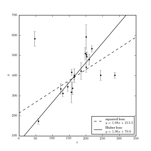
Figure 8.8

An example of fitting a simple linear model to data which includes outliers (data is from table 1 of Hogg et al 2010). A comparison of linear regression using the squared-loss function (equivalent to ordinary least-squares regression) and the Huber loss function, with c = 1 (i.e., beyond 1 standard deviation, the loss becomes linear).

Code output:

Optimization terminated successfully.
         Current function value: 289.963723
         Iterations: 62
         Function evaluations: 117
Optimization terminated successfully.
         Current function value: 43.439758
         Iterations: 59
         Function evaluations: 115
[   1.07674745  213.27350923]
[  1.96473118  70.00573832]

Python source code:

# Author: Jake VanderPlas
# License: BSD
#   The figure produced by this code is published in the textbook
#   "Statistics, Data Mining, and Machine Learning in Astronomy" (2013)
#   For more information, see http://astroML.github.com
#   To report a bug or issue, use the following forum:
#    https://groups.google.com/forum/#!forum/astroml-general
import numpy as np
from matplotlib import pyplot as plt

from scipy import optimize
from astroML.datasets import fetch_hogg2010test

#----------------------------------------------------------------------
# This function adjusts matplotlib settings for a uniform feel in the textbook.
# Note that with usetex=True, fonts are rendered with LaTeX.  This may
# result in an error if LaTeX is not installed on your system.  In that case,
# you can set usetex to False.
from astroML.plotting import setup_text_plots
setup_text_plots(fontsize=8, usetex=True)

#------------------------------------------------------------
# Get data: this includes outliers
data = fetch_hogg2010test()
x = data['x']
y = data['y']
dy = data['sigma_y']


# Define the standard squared-loss function
def squared_loss(m, b, x, y, dy):
    y_fit = m * x + b
    return np.sum(((y - y_fit) / dy) ** 2, -1)


# Define the log-likelihood via the Huber loss function
def huber_loss(m, b, x, y, dy, c=2):
    y_fit = m * x + b
    t = abs((y - y_fit) / dy)
    flag = t > c
    return np.sum((~flag) * (0.5 * t ** 2) - (flag) * c * (0.5 * c - t), -1)

f_squared = lambda beta: squared_loss(beta[0], beta[1], x=x, y=y, dy=dy)
f_huber = lambda beta: huber_loss(beta[0], beta[1], x=x, y=y, dy=dy, c=1)

#------------------------------------------------------------
# compute the maximum likelihood using the huber loss
beta0 = (2, 30)
beta_squared = optimize.fmin(f_squared, beta0)
beta_huber = optimize.fmin(f_huber, beta0)

print beta_squared
print beta_huber

#------------------------------------------------------------
# Plot the results
fig = plt.figure(figsize=(5, 5))
ax = fig.add_subplot(111)

x_fit = np.linspace(0, 350, 10)
ax.plot(x_fit, beta_squared[0] * x_fit + beta_squared[1], '--k',
        label="squared loss:\n $y=%.2fx + %.1f$" % tuple(beta_squared))
ax.plot(x_fit, beta_huber[0] * x_fit + beta_huber[1], '-k',
        label="Huber loss:\n $y=%.2fx + %.1f$" % tuple(beta_huber))
ax.legend(loc=4)

ax.errorbar(x, y, dy, fmt='.k', lw=1, ecolor='gray')

ax.set_xlim(0, 350)
ax.set_ylim(100, 700)
ax.set_xlabel('$x$')
ax.set_ylabel('$y$')

plt.show()

[download source: fig_huber_loss.py]