Cosmology Regression Example

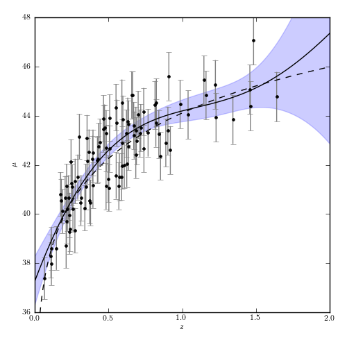
Figure 8.11

A Gaussian process regression analysis of the simulated supernova sample used in figure 8.2. This uses a squared-exponential covariance model, with bandwidth learned through cross-validation.

Code output:

[[ 0.18093568]]

Python source code:

# Author: Jake VanderPlas
# License: BSD
#   The figure produced by this code is published in the textbook
#   "Statistics, Data Mining, and Machine Learning in Astronomy" (2013)
#   For more information, see http://astroML.github.com
#   To report a bug or issue, use the following forum:
#    https://groups.google.com/forum/#!forum/astroml-general
import numpy as np
from matplotlib import pyplot as plt

from sklearn.gaussian_process import GaussianProcess

from astroML.cosmology import Cosmology
from astroML.datasets import generate_mu_z

#----------------------------------------------------------------------
# This function adjusts matplotlib settings for a uniform feel in the textbook.
# Note that with usetex=True, fonts are rendered with LaTeX.  This may
# result in an error if LaTeX is not installed on your system.  In that case,
# you can set usetex to False.
from astroML.plotting import setup_text_plots
setup_text_plots(fontsize=8, usetex=True)

#------------------------------------------------------------
# Generate data
z_sample, mu_sample, dmu = generate_mu_z(100, random_state=0)

cosmo = Cosmology()
z = np.linspace(0.01, 2, 1000)
mu_true = np.asarray(map(cosmo.mu, z))

#------------------------------------------------------------
# fit the data
# Mesh the input space for evaluations of the real function,
# the prediction and its MSE
z_fit = np.linspace(0, 2, 1000)
gp = GaussianProcess(corr='squared_exponential', theta0=1e-1,
                     thetaL=1e-2, thetaU=1,
                     normalize=False,
                     nugget=(dmu / mu_sample) ** 2,
                     random_start=1)
gp.fit(z_sample[:, None], mu_sample)
y_pred, MSE = gp.predict(z_fit[:, None], eval_MSE=True)
sigma = np.sqrt(MSE)
print gp.theta_


#------------------------------------------------------------
# Plot the gaussian process
#  gaussian process allows computation of the error at each point
#  so we will show this as a shaded region
fig = plt.figure(figsize=(5, 5))
fig.subplots_adjust(left=0.1, right=0.95, bottom=0.1, top=0.95)
ax = fig.add_subplot(111)

ax.plot(z, mu_true, '--k')
ax.errorbar(z_sample, mu_sample, dmu, fmt='.k', ecolor='gray', markersize=6)
ax.plot(z_fit, y_pred, '-k')
ax.fill_between(z_fit, y_pred - 1.96 * sigma, y_pred + 1.96 * sigma,
                alpha=0.2, color='b', label='95% confidence interval')

ax.set_xlabel('$z$')
ax.set_ylabel(r'$\mu$')

ax.set_xlim(0, 2)
ax.set_ylim(36, 48)

plt.show()

[download source: fig_gp_mu_z.py]