Cross Validation Examples: Part 1

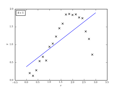
Figure 8.12

Our toy data set described by eq. 8.75. Shown is the line of best fit, which quite clearly underfits the data. In other words, a linear model in this case has high bias.

Code output:

Python source code:

# Author: Jake VanderPlas
# License: BSD
#   The figure produced by this code is published in the textbook
#   "Statistics, Data Mining, and Machine Learning in Astronomy" (2013)
#   For more information, see http://astroML.github.com
#   To report a bug or issue, use the following forum:
#    https://groups.google.com/forum/#!forum/astroml-general
import numpy as np
from matplotlib import pyplot as plt
from matplotlib import ticker
from matplotlib.patches import FancyArrow

#----------------------------------------------------------------------
# This function adjusts matplotlib settings for a uniform feel in the textbook.
# Note that with usetex=True, fonts are rendered with LaTeX.  This may
# result in an error if LaTeX is not installed on your system.  In that case,
# you can set usetex to False.
from astroML.plotting import setup_text_plots
setup_text_plots(fontsize=8, usetex=True)


#------------------------------------------------------------
# Define our functional form
def func(x, dy=0.1):
    return np.random.normal(np.sin(x) * x, dy)

#------------------------------------------------------------
# select the (noisy) data
np.random.seed(0)
x = np.linspace(0, 3, 22)[1:-1]
dy = 0.1
y = func(x, dy)

#------------------------------------------------------------
# Select the cross-validation points
np.random.seed(1)
x_cv = 3 * np.random.random(20)
y_cv = func(x_cv)

x_fit = np.linspace(0, 3, 1000)

#------------------------------------------------------------
# First figure: plot points with a linear fit
fig = plt.figure(figsize=(5, 3.75))
ax = fig.add_subplot(111)

ax.scatter(x, y, marker='x', c='k', s=30)

p = np.polyfit(x, y, 1)
y_fit = np.polyval(p, x_fit)

ax.text(0.03, 0.96, "d = 1", transform=plt.gca().transAxes,
        ha='left', va='top',
        bbox=dict(ec='k', fc='w', pad=10))

ax.plot(x_fit, y_fit, '-b')
ax.set_xlabel('$x$')
ax.set_ylabel('$y$')

plt.show()

[download source: fig_cross_val_A.py]