Scematic Diagram of PCA

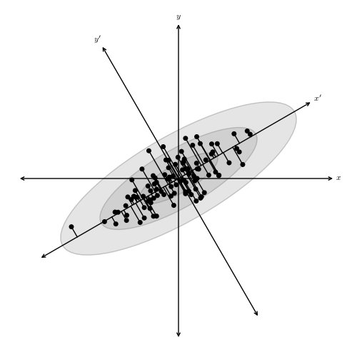
Figure 7.2

A distribution of points drawn from a bivariate Gaussian and centered on the origin of x and y. PCA defines a rotation such that the new axes (x’ and y’) are aligned along the directions of maximal variance (the principal components) with zero covariance. This is equivalent to minimizing the square of the perpendicular distances between the points and the principal components.

Code output:

Python source code:

# Author: Jake VanderPlas
# License: BSD
#   The figure produced by this code is published in the textbook
#   "Statistics, Data Mining, and Machine Learning in Astronomy" (2013)
#   For more information, see http://astroML.github.com
#   To report a bug or issue, use the following forum:
#    https://groups.google.com/forum/#!forum/astroml-general
import numpy as np
from matplotlib import pyplot as plt
from matplotlib.patches import Ellipse

#----------------------------------------------------------------------
# This function adjusts matplotlib settings for a uniform feel in the textbook.
# Note that with usetex=True, fonts are rendered with LaTeX.  This may
# result in an error if LaTeX is not installed on your system.  In that case,
# you can set usetex to False.
from astroML.plotting import setup_text_plots
setup_text_plots(fontsize=8, usetex=True)

#------------------------------------------------------------
# Set parameters and draw the random sample
np.random.seed(42)
r = 0.9

sigma1 = 0.25
sigma2 = 0.08
rotation = np.pi / 6
s = np.sin(rotation)
c = np.cos(rotation)

X = np.random.normal(0, [sigma1, sigma2], size=(100, 2)).T
R = np.array([[c, -s],
              [s, c]])
X = np.dot(R, X)

#------------------------------------------------------------
# Plot the diagram
fig = plt.figure(figsize=(5, 5), facecolor='w')
ax = plt.axes((0, 0, 1, 1), xticks=[], yticks=[], frameon=False)

# draw axes
ax.annotate(r'$x$', (-r, 0), (r, 0),
            ha='center', va='center',
            arrowprops=dict(arrowstyle='<->', color='k', lw=1))
ax.annotate(r'$y$', (0, -r), (0, r),
            ha='center', va='center',
            arrowprops=dict(arrowstyle='<->', color='k', lw=1))

# draw rotated axes
ax.annotate(r'$x^\prime$', (-r * c, -r * s), (r * c, r * s),
            ha='center', va='center',
            arrowprops=dict(color='k', arrowstyle='<->', lw=1))
ax.annotate(r'$y^\prime$', (r * s, -r * c), (-r * s, r * c),
            ha='center', va='center',
            arrowprops=dict(color='k', arrowstyle='<->', lw=1))

# scatter points
ax.scatter(X[0], X[1], s=25, lw=0, c='k', zorder=2)

# draw lines
vnorm = np.array([s, -c])
for v in (X.T):
    d = np.dot(v, vnorm)
    v1 = v - d * vnorm
    ax.plot([v[0], v1[0]], [v[1], v1[1]], '-k')

# draw ellipses
for sigma in (1, 2, 3):
    ax.add_patch(Ellipse((0, 0), 2 * sigma * sigma1, 2 * sigma * sigma2,
                         rotation * 180. / np.pi,
                         ec='k', fc='gray', alpha=0.2, zorder=1))

ax.set_xlim(-1, 1)
ax.set_ylim(-1, 1)

plt.show()

[download source: fig_PCA_rotation.py]