Binomial Posterior

Figure 5.9

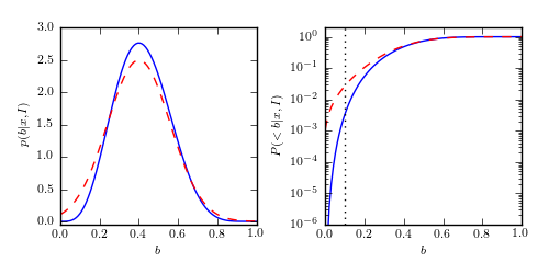
The solid line in the left panel shows the posterior pdf p(b|k, N) described by eq. 5.71, for k = 4 and N = 10. The dashed line shows a Gaussian approximation described in Section 3.3.3. The right panel shows the corresponding cumulative distributions. A value of 0.1 is marginally likely according to the Gaussian approximation (p_approx(< 0.1) ~ 0.03) but strongly rejected by the true distribution (p_true(< 0.1) ~ 0.003).

Code output:

Python source code:

# Author: Jake VanderPlas
# License: BSD
#   The figure produced by this code is published in the textbook
#   "Statistics, Data Mining, and Machine Learning in Astronomy" (2013)
#   For more information, see http://astroML.github.com
#   To report a bug or issue, use the following forum:
#    https://groups.google.com/forum/#!forum/astroml-general
import numpy as np
from scipy.stats import norm, binom
from matplotlib import pyplot as plt

#----------------------------------------------------------------------
# This function adjusts matplotlib settings for a uniform feel in the textbook.
# Note that with usetex=True, fonts are rendered with LaTeX.  This may
# result in an error if LaTeX is not installed on your system.  In that case,
# you can set usetex to False.
from astroML.plotting import setup_text_plots
setup_text_plots(fontsize=8, usetex=True)

#------------------------------------------------------------
# Plot posterior as a function of b
n = 10  # number of points
k = 4   # number of successes from n draws

b = np.linspace(0, 1, 100)
db = b[1] - b[0]

# compute the probability p(b) (eqn. 5.70)
p_b = b ** k * (1 - b) ** (n - k)
p_b /= p_b.sum()
p_b /= db
cuml_p_b = p_b.cumsum()
cuml_p_b /= cuml_p_b[-1]

# compute the gaussian approximation (eqn. 5.71)
p_g = norm(k * 1. / n, 0.16).pdf(b)
cuml_p_g = p_g.cumsum()
cuml_p_g /= cuml_p_g[-1]

#------------------------------------------------------------
# Plot the results
fig = plt.figure(figsize=(5, 2.5))
fig.subplots_adjust(left=0.11, right=0.95, wspace=0.35, bottom=0.18)

ax = fig.add_subplot(121)
ax.plot(b, p_b, '-b')
ax.plot(b, p_g, '--r')

ax.set_ylim(-0.05, 3)

ax.set_xlabel('$b$')
ax.set_ylabel('$p(b|x,I)$')

ax = fig.add_subplot(122, yscale='log')
ax.plot(b, cuml_p_b, '-b')
ax.plot(b, cuml_p_g, '--r')
ax.plot([0.1, 0.1], [1E-6, 2], ':k')

ax.set_xlabel('$b$')
ax.set_ylabel('$P(<b|x,I)$')
ax.set_ylim(1E-6, 2)

plt.show()

[download source: fig_posterior_binomial.py]