Gaussian Distribution with Gaussian Errors

Figure 5.7

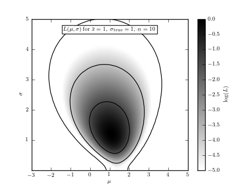
The logarithm of the posterior probability density function for and , , for a Gaussian distribution with heteroscedastic Gaussian measurement errors (sampled uniformly from the 0-3 interval), given by eq. 5.64. The input values are and , and a randomly generated sample has 10 points. Note that the posterior pdf is not symmetric with respect to the line, and that the outermost contour, which encloses the region that contains 0.997 of the cumulative (integrated) posterior probability, allows solutions with .

Code output:

Python source code:

# Author: Jake VanderPlas
# License: BSD
#   The figure produced by this code is published in the textbook
#   "Statistics, Data Mining, and Machine Learning in Astronomy" (2013)
#   For more information, see http://astroML.github.com
#   To report a bug or issue, use the following forum:
#    https://groups.google.com/forum/#!forum/astroml-general
import numpy as np
from matplotlib import pyplot as plt
from astroML.plotting.mcmc import convert_to_stdev

#----------------------------------------------------------------------
# This function adjusts matplotlib settings for a uniform feel in the textbook.
# Note that with usetex=True, fonts are rendered with LaTeX.  This may
# result in an error if LaTeX is not installed on your system.  In that case,
# you can set usetex to False.
from astroML.plotting import setup_text_plots
setup_text_plots(fontsize=8, usetex=True)


def gaussgauss_logL(xi, ei, mu, sigma):
    """Equation 5.63: gaussian likelihood with gaussian errors"""
    ndim = len(np.broadcast(sigma, mu).shape)

    xi = xi.reshape(xi.shape + tuple(ndim * [1]))
    ei = ei.reshape(ei.shape + tuple(ndim * [1]))

    s2_e2 = sigma ** 2 + ei ** 2
    return -0.5 * np.sum(np.log(s2_e2) + (xi - mu) ** 2 / s2_e2, 0)

#------------------------------------------------------------
# Define the grid and compute logL
np.random.seed(5)
mu_true = 1.
sigma_true = 1.
N = 10
ei = 3 * np.random.random(N)
xi = np.random.normal(mu_true, np.sqrt(sigma_true ** 2 + ei ** 2))

sigma = np.linspace(0.01, 5, 70)
mu = np.linspace(-3, 5, 70)

logL = gaussgauss_logL(xi, ei, mu, sigma[:, np.newaxis])
logL -= logL.max()

#------------------------------------------------------------
# plot the results
fig = plt.figure(figsize=(5, 3.75))
plt.imshow(logL, origin='lower',
           extent=(mu[0], mu[-1], sigma[0], sigma[-1]),
           cmap=plt.cm.binary,
           aspect='auto')
plt.colorbar().set_label(r'$\log(L)$')
plt.clim(-5, 0)

plt.text(0.5, 0.93,
         (r'$L(\mu,\sigma)\ \mathrm{for}\ \bar{x}=1,\ '
          r'\sigma_{\rm true}=1,\ n=10$'),
         bbox=dict(ec='k', fc='w', alpha=0.9),
         ha='center', va='center', transform=plt.gca().transAxes)

plt.contour(mu, sigma, convert_to_stdev(logL),
            levels=(0.683, 0.955, 0.997),
            colors='k')

plt.xlabel(r'$\mu$')
plt.ylabel(r'$\sigma$')

plt.show()

[download source: fig_likelihood_gaussgauss.py]