Gaussian/Gaussian distribution

Figure 5.6

The distribution of 106 points drawn from and sampled with heteroscedastic Gaussian errors with widths, , uniformly distributed between 0 and 3. A linear superposition of these Gaussian distributions with widths equal to sigma_G` (eq.3.36) are shown for comparison.

Code output:

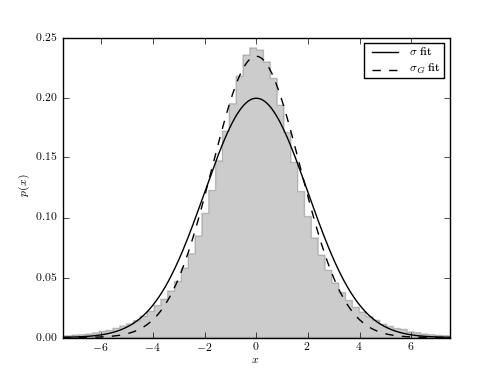
anderson-darling A^2 = 3088.1

Python source code:

# Author: Jake VanderPlas
# License: BSD
#   The figure produced by this code is published in the textbook
#   "Statistics, Data Mining, and Machine Learning in Astronomy" (2013)
#   For more information, see http://astroML.github.com
#   To report a bug or issue, use the following forum:
#    https://groups.google.com/forum/#!forum/astroml-general
import numpy as np
from matplotlib import pyplot as plt
from scipy.stats import norm, anderson
from astroML.stats import mean_sigma, median_sigmaG

#----------------------------------------------------------------------
# This function adjusts matplotlib settings for a uniform feel in the textbook.
# Note that with usetex=True, fonts are rendered with LaTeX.  This may
# result in an error if LaTeX is not installed on your system.  In that case,
# you can set usetex to False.
from astroML.plotting import setup_text_plots
setup_text_plots(fontsize=8, usetex=True)

#------------------------------------------------------------
# Create distributions

# draw underlying points
np.random.seed(0)
Npts = 1E6
x = np.random.normal(loc=0, scale=1, size=Npts)

# add error for each point
e = 3 * np.random.random(Npts)
x += np.random.normal(0, e)

# compute anderson-darling test
A2, sig, crit = anderson(x)
print "anderson-darling A^2 = %.1f" % A2

# compute point statistics
mu_sample, sig_sample = mean_sigma(x, ddof=1)
med_sample, sigG_sample = median_sigmaG(x)

#------------------------------------------------------------
# plot the results
fig, ax = plt.subplots(figsize=(5, 3.75))
ax.hist(x, 100, histtype='stepfilled', alpha=0.2,
        color='k', normed=True)

# plot the fitting normal curves
x_sample = np.linspace(-15, 15, 1000)
ax.plot(x_sample, norm(mu_sample, sig_sample).pdf(x_sample),
        '-k', label='$\sigma$ fit')
ax.plot(x_sample, norm(med_sample, sigG_sample).pdf(x_sample),
        '--k', label='$\sigma_G$ fit')
ax.legend()

ax.set_xlim(-7.5, 7.5)
ax.set_xlabel('$x$')
ax.set_ylabel('$p(x)$')
plt.show()

[download source: fig_distribution_gaussgauss.py]