Distribution Representation Comparison

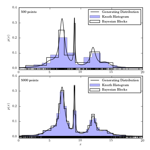
Figure 5.21

Comparison of Knuth’s histogram and a Bayesian blocks histogram. The adaptive bin widths of the Bayesian blocks histogram yield a better representation of the underlying data, especially with fewer points.

Code output:

Optimization terminated successfully.
         Current function value: -347.779301
         Iterations: 16
         Function evaluations: 45
Optimization terminated successfully.
         Current function value: -5779.829570
         Iterations: 17
         Function evaluations: 48

Python source code:

# Author: Jake VanderPlas
# License: BSD
#   The figure produced by this code is published in the textbook
#   "Statistics, Data Mining, and Machine Learning in Astronomy" (2013)
#   For more information, see http://astroML.github.com
#   To report a bug or issue, use the following forum:
#    https://groups.google.com/forum/#!forum/astroml-general
import numpy as np
from matplotlib import pyplot as plt
from scipy import stats

from astroML.plotting import hist

#----------------------------------------------------------------------
# This function adjusts matplotlib settings for a uniform feel in the textbook.
# Note that with usetex=True, fonts are rendered with LaTeX.  This may
# result in an error if LaTeX is not installed on your system.  In that case,
# you can set usetex to False.
from astroML.plotting import setup_text_plots
setup_text_plots(fontsize=8, usetex=True)

#------------------------------------------------------------
# Generate our data: a mix of several Cauchy distributions
np.random.seed(0)
N = 10000
mu_gamma_f = [(5, 1.0, 0.1),
              (7, 0.5, 0.5),
              (9, 0.1, 0.1),
              (12, 0.5, 0.2),
              (14, 1.0, 0.1)]
true_pdf = lambda x: sum([f * stats.cauchy(mu, gamma).pdf(x)
                          for (mu, gamma, f) in mu_gamma_f])
x = np.concatenate([stats.cauchy(mu, gamma).rvs(int(f * N))
                    for (mu, gamma, f) in mu_gamma_f])
np.random.shuffle(x)
x = x[x > -10]
x = x[x < 30]

#------------------------------------------------------------
# plot the results
fig = plt.figure(figsize=(5, 5))
fig.subplots_adjust(bottom=0.08, top=0.95, right=0.95, hspace=0.1)
N_values = (500, 5000)
subplots = (211, 212)

for N, subplot in zip(N_values, subplots):
    ax = fig.add_subplot(subplot)
    xN = x[:N]
    t = np.linspace(-10, 30, 1000)

    # plot the results
    ax.plot(xN, -0.005 * np.ones(len(xN)), '|k')
    hist(xN, bins='knuth', ax=ax, normed=True,
         histtype='stepfilled', alpha=0.3,
         label='Knuth Histogram')
    hist(xN, bins='blocks', ax=ax, normed=True,
         histtype='step', color='k',
         label="Bayesian Blocks")
    ax.plot(t, true_pdf(t), '-', color='black',
            label="Generating Distribution")

    # label the plot
    ax.text(0.02, 0.95, "%i points" % N, ha='left', va='top',
            transform=ax.transAxes)
    ax.set_ylabel('$p(x)$')
    ax.legend(loc='upper right', prop=dict(size=8))

    if subplot == 212:
        ax.set_xlabel('$x$')

    ax.set_xlim(0, 20)
    ax.set_ylim(-0.01, 0.4001)

plt.show()

[download source: fig_bayes_blocks.py]