Plot a Diagram explaining a Convolution

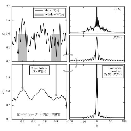
Figure 10.2

A schematic of how the convolution of two functions works. The top-left panel shows simulated data (black line); this time series is convolved with a top-hat function (gray boxes); see eq. 10.8. The top-right panels show the Fourier transform of the data and the window function. These can be multiplied together (bottom-right panel) and inverse transformed to find the convolution (bottom-left panel), which amounts to integrating the data over copies of the window at all locations. The result in the bottom-left panel can be viewed as the signal shown in the top-left panel smoothed with the window (top-hat) function.

Code output:

Python source code:

# Author: Jake VanderPlas
# License: BSD
#   The figure produced by this code is published in the textbook
#   "Statistics, Data Mining, and Machine Learning in Astronomy" (2013)
#   For more information, see http://astroML.github.com
#   To report a bug or issue, use the following forum:
#    https://groups.google.com/forum/#!forum/astroml-general
import numpy as np
from matplotlib import pyplot as plt

from scipy.signal import fftconvolve

#----------------------------------------------------------------------
# This function adjusts matplotlib settings for a uniform feel in the textbook.
# Note that with usetex=True, fonts are rendered with LaTeX.  This may
# result in an error if LaTeX is not installed on your system.  In that case,
# you can set usetex to False.
from astroML.plotting import setup_text_plots
setup_text_plots(fontsize=8, usetex=True)

#------------------------------------------------------------
# Generate random x, y with a given covariance length
np.random.seed(1)
x = np.linspace(0, 1, 500)
h = 0.01
C = np.exp(-0.5 * (x - x[:, None]) ** 2 / h ** 2)
y = 0.8 + 0.3 * np.random.multivariate_normal(np.zeros(len(x)), C)

#------------------------------------------------------------
# Define a normalized top-hat window function
w = np.zeros_like(x)
w[(x > 0.12) & (x < 0.28)] = 1

#------------------------------------------------------------
# Perform the convolution
y_norm = np.convolve(np.ones_like(y), w, mode='full')
valid_indices = (y_norm != 0)
y_norm = y_norm[valid_indices]

y_w = np.convolve(y, w, mode='full')[valid_indices] / y_norm

# trick: convolve with x-coordinate to find the center of the window at
#        each point.
x_w = np.convolve(x, w, mode='full')[valid_indices] / y_norm

#------------------------------------------------------------
# Compute the Fourier transforms of the signal and window
y_fft = np.fft.fft(y)
w_fft = np.fft.fft(w)

yw_fft = y_fft * w_fft
yw_final = np.fft.ifft(yw_fft)

#------------------------------------------------------------
# Set up the plots
fig = plt.figure(figsize=(5, 5))
fig.subplots_adjust(left=0.09, bottom=0.09, right=0.95, top=0.95,
                    hspace=0.05, wspace=0.05)

#----------------------------------------
# plot the data and window function
ax = fig.add_subplot(221)
ax.plot(x, y, '-k', label=r'data $D(x)$')
ax.fill(x, w, color='gray', alpha=0.5,
        label=r'window $W(x)$')
ax.fill(x, w[::-1], color='gray', alpha=0.5)

ax.legend()
ax.xaxis.set_major_formatter(plt.NullFormatter())

ax.set_ylabel('$D$')

ax.set_xlim(0.01, 0.99)
ax.set_ylim(0, 2.0)

#----------------------------------------
# plot the convolution
ax = fig.add_subplot(223)
ax.plot(x_w, y_w, '-k')

ax.text(0.5, 0.95, "Convolution:\n" + r"$[D \ast W](x)$",
        ha='center', va='top', transform=ax.transAxes,
        bbox=dict(fc='w', ec='k', pad=8), zorder=2)

ax.text(0.5, 0.05,
        (r'$[D \ast W](x)$' +
         r'$= \mathcal{F}^{-1}\{\mathcal{F}[D] \cdot \mathcal{F}[W]\}$'),
        ha='center', va='bottom', transform=ax.transAxes)

for x_loc in (0.2, 0.8):
    y_loc = y_w[x_w <= x_loc][-1]
    ax.annotate('', (x_loc, y_loc), (x_loc, 2.0), zorder=1,
                arrowprops=dict(arrowstyle='->', color='gray', lw=2))

ax.set_xlabel('$x$')
ax.set_ylabel('$D_W$')

ax.set_xlim(0.01, 0.99)
ax.set_ylim(0, 1.99)

#----------------------------------------
# plot the Fourier transforms
N = len(x)
k = - 0.5 * N + np.arange(N) * 1. / N / (x[1] - x[0])

ax = fig.add_subplot(422)
ax.plot(k, abs(np.fft.fftshift(y_fft)), '-k')

ax.text(0.95, 0.95, r'$\mathcal{F}(D)$',
        ha='right', va='top', transform=ax.transAxes)

ax.set_xlim(-100, 100)
ax.set_ylim(-5, 85)

ax.xaxis.set_major_formatter(plt.NullFormatter())
ax.yaxis.set_major_formatter(plt.NullFormatter())

ax = fig.add_subplot(424)
ax.plot(k, abs(np.fft.fftshift(w_fft)), '-k')

ax.text(0.95, 0.95,  r'$\mathcal{F}(W)$', ha='right', va='top',
        transform=ax.transAxes)

ax.set_xlim(-100, 100)
ax.set_ylim(-5, 85)

ax.xaxis.set_major_formatter(plt.NullFormatter())
ax.yaxis.set_major_formatter(plt.NullFormatter())

#----------------------------------------
# plot the product of Fourier transforms
ax = fig.add_subplot(224)
ax.plot(k, abs(np.fft.fftshift(yw_fft)), '-k')

ax.text(0.95, 0.95, ('Pointwise\nproduct:\n' +
                     r'$\mathcal{F}(D) \cdot \mathcal{F}(W)$'),
        ha='right', va='top', transform=ax.transAxes,
        bbox=dict(fc='w', ec='k', pad=8), zorder=2)

ax.set_xlim(-100, 100)
ax.set_ylim(-100, 3500)

ax.set_xlabel('$k$')

ax.yaxis.set_major_formatter(plt.NullFormatter())

#------------------------------------------------------------
# Plot flow arrows
ax = fig.add_axes([0, 0, 1, 1], xticks=[], yticks=[], frameon=False)

arrowprops = dict(arrowstyle="simple",
                  color="gray", alpha=0.5,
                  shrinkA=5, shrinkB=5,
                  patchA=None,
                  patchB=None,
                  connectionstyle="arc3,rad=-0.35")

ax.annotate('', [0.57, 0.57], [0.47, 0.57],
            arrowprops=arrowprops,
            transform=ax.transAxes)
ax.annotate('', [0.57, 0.47], [0.57, 0.57],
            arrowprops=arrowprops,
            transform=ax.transAxes)
ax.annotate('', [0.47, 0.47], [0.57, 0.47],
            arrowprops=arrowprops,
            transform=ax.transAxes)

plt.show()

[download source: fig_convolution_diagram.py]