SDSS Stripe 82 Standard Stars

Figure 1.9.

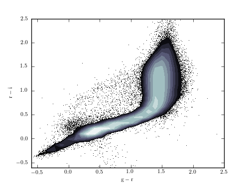
Scatter plot with contours over dense regions.This is a color-color diagram of the entire set of SDSS Stripe 82 standard stars; cf. figure 1.6.

Code output:

Python source code:

# Author: Jake VanderPlas
# License: BSD
#   The figure produced by this code is published in the textbook
#   "Statistics, Data Mining, and Machine Learning in Astronomy" (2013)
#   For more information, see http://astroML.github.com
#   To report a bug or issue, use the following forum:
#    https://groups.google.com/forum/#!forum/astroml-general
from matplotlib import pyplot as plt

from astroML.plotting import scatter_contour
from astroML.datasets import fetch_sdss_S82standards

#----------------------------------------------------------------------
# This function adjusts matplotlib settings for a uniform feel in the textbook.
# Note that with usetex=True, fonts are rendered with LaTeX.  This may
# result in an error if LaTeX is not installed on your system.  In that case,
# you can set usetex to False.
from astroML.plotting import setup_text_plots
setup_text_plots(fontsize=8, usetex=True)

#------------------------------------------------------------
# Fetch the Stripe 82 standard star catalog

data = fetch_sdss_S82standards()

g = data['mmu_g']
r = data['mmu_r']
i = data['mmu_i']

#------------------------------------------------------------
# plot the results
fig, ax = plt.subplots(figsize=(5, 3.75))
scatter_contour(g - r, r - i, threshold=200, log_counts=True, ax=ax,
                histogram2d_args=dict(bins=40),
                plot_args=dict(marker=',', linestyle='none', color='black'),
                contour_args=dict(cmap=plt.cm.bone))

ax.set_xlabel(r'${\rm g - r}$')
ax.set_ylabel(r'${\rm r - i}$')

ax.set_xlim(-0.6, 2.5)
ax.set_ylim(-0.6, 2.5)

plt.show()

[download source: fig_S82_scatter_contour.py]