Finding a signal in a background
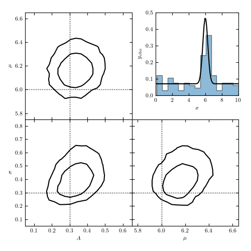
Figure 5.26
Fitting a model of a signal in an unknown background. The histogram in the top-right panel visualizes a sample drawn from a Gaussian signal plus a uniform background model given by eq. 5.83 and shown by the line. The remaining panels show projections of the three-dimensional posterior pdf, based on a 20,000 point MCMC chain.
# Author: Jake VanderPlas (adapted to PyMC3 by Brigitta Sipocz)
# License: BSD
#   The figure produced by this code is published in the textbook
#   "Statistics, Data Mining, and Machine Learning in Astronomy" (2013)
#   For more information, see http://astroML.github.com
#   To report a bug or issue, use the following forum:
#    https://groups.google.com/forum/#!forum/astroml-general
import numpy as np
from matplotlib import pyplot as plt
from scipy import stats

import pymc3 as pm
import theano.tensor as tt

from astroML.plotting import plot_mcmc

# ----------------------------------------------------------------------
# This function adjusts matplotlib settings for a uniform feel in the textbook.
# Note that with usetex=True, fonts are rendered with LaTeX.  This may
# result in an error if LaTeX is not installed on your system.  In that case,
# you can set usetex to False.
if "setup_text_plots" not in globals():
    from astroML.plotting import setup_text_plots
setup_text_plots(fontsize=8, usetex=True)

# ----------------------------------------------------------------------
# Set up dataset: gaussian signal in a uniform background
np.random.seed(0)

N = 100

A_true = 0.3
W_true = 10
x0_true = 6
sigma_true = 0.3

signal = stats.norm(x0_true, sigma_true)
background = stats.uniform(0, W_true)

x = np.random.random(N)
i_sig = x < A_true
i_bg = ~i_sig
x[i_sig] = signal.rvs(np.sum(i_sig))
x[i_bg] = background.rvs(np.sum(i_bg))


# ----------------------------------------------------------------------
# Set up MCMC sampling
with pm.Model():
    A = pm.Uniform('A', 0, 1)
    x0 = pm.Uniform('x0', 0, 10)
    log_sigma = pm.Uniform('log_sigma', -5, 5)

    def sigbg_like(x):
        """signal + background likelihood"""
        sigma = np.exp(log_sigma)
        return tt.sum(np.log(A * np.exp(-0.5 * ((x - x0) / sigma) ** 2)
                             / np.sqrt(2 * np.pi) / sigma + (1 - A) / W_true))

    SigBG = pm.DensityDist('sigbg',
                           logp=sigbg_like,
                           observed=x)
    trace = pm.sample(draws=5000, tune=1000)

# ------------------------------------------------------------
# Plot the results
fig = plt.figure(figsize=(5, 5))
ax_list = plot_mcmc([trace[s] for s in ['A', 'x0']] + [np.exp(trace['log_sigma']),],
                    limits=[(0.05, 0.65), (5.75, 6.65), (0.05, 0.85)],
                    labels=[r'$A$', r'$\mu$', r'$\sigma$'],
                    bounds=(0.1, 0.1, 0.95, 0.95),
                    true_values=[A_true, x0_true, sigma_true],
                    fig=fig, colors='k')

ax = plt.axes([0.62, 0.62, 0.33, 0.33])
x_pdf = np.linspace(0, 10, 100)
y_pdf = A_true * signal.pdf(x_pdf) + (1 - A_true) * background.pdf(x_pdf)

ax.hist(x, 15, density=True, histtype='stepfilled', alpha=0.5)
ax.plot(x_pdf, y_pdf, '-k')

ax.set_xlim(0, 10)
ax.set_ylim(0, 0.5)
ax.set_xlabel('$x$')
ax.set_ylabel(r'$y_{\rm obs}$')

plt.show()