Gaussian Distribution with Gaussian Errors

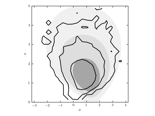
Figure 5.25

The posterior pdf for mu and sigma for a Gaussian distribution with heteroscedastic errors. This is the same data set as used in figure 5.7, but here each measurement error is assumed unknown, treated as a model parameter with a scale-invariant prior, and marginalized over to obtain the distribution of mu and sigma shown by contours. For comparison, the posterior pdf from figure 5.7 is shown by shaded contours.

Code output:

Python source code:

# Author: Jake VanderPlas (adapted to PyMC3 by Brigitta Sipocz)
# License: BSD
#   The figure produced by this code is published in the textbook
#   "Statistics, Data Mining, and Machine Learning in Astronomy" (2013)
#   For more information, see http://astroML.github.com
#   To report a bug or issue, use the following forum:
#    https://groups.google.com/forum/#!forum/astroml-general
import numpy as np
from matplotlib import pyplot as plt

import pymc3 as pm

from astroML.plotting.mcmc import convert_to_stdev
from astroML.plotting import plot_mcmc

# ----------------------------------------------------------------------
# This function adjusts matplotlib settings for a uniform feel in the textbook.
# Note that with usetex=True, fonts are rendered with LaTeX.  This may
# result in an error if LaTeX is not installed on your system.  In that case,
# you can set usetex to False.
if "setup_text_plots" not in globals():
    from astroML.plotting import setup_text_plots
setup_text_plots(fontsize=8, usetex=True)


def gaussgauss_logL(xi, ei, mu, sigma):
    """Equation 5.22: gaussian likelihood"""
    ndim = len(np.broadcast(sigma, mu).shape)

    xi = xi.reshape(xi.shape + tuple(ndim * [1]))
    ei = ei.reshape(ei.shape + tuple(ndim * [1]))

    s2_e2 = sigma ** 2 + ei ** 2
    return -0.5 * np.sum(np.log(s2_e2) + (xi - mu) ** 2 / s2_e2, 0)


# ------------------------------------------------------------
# Select the data
np.random.seed(5)
mu_true = 1.
sigma_true = 1.
N = 10
ei = 3 * np.random.random(N)
xi = np.random.normal(mu_true, np.sqrt(sigma_true ** 2 + ei ** 2))

# ----------------------------------------------------------------------
# Set up MCMC for our model parameters: (mu, sigma, ei)
with pm.Model() as model:
    mu = pm.Uniform('mu', -10, 10)
    log_sigma = pm.Uniform('log_sigma', -10, 10)
    log_error = pm.Uniform('log_error', -10, 10, shape=(N,))

    def sigma_m(log_sigma, log_error):
        return np.sqrt(np.exp(log_sigma) ** 2 + np.exp(log_error)**2)

    x = pm.Normal('x', mu=mu, sd=sigma_m(log_sigma, log_error), observed=xi)

    # perform the MCMC sampling
    trace = pm.sample(draws=4500, tune=1500)

# ------------------------------------------------------------
# Extract the MCMC traces

fig = plt.figure(figsize=(5, 3.75))
ax, = plot_mcmc([trace['mu'], np.exp(trace['log_sigma'])], fig=fig,
                limits=[(-3.2, 4.2), (0, 5)],
                bounds=(0.08, 0.12, 0.95, 0.95),
                labels=(r'$\mu$', r'$\sigma$'),
                levels=[0.683, 0.955, 0.997],
                colors='k')

# ----------------------------------------------------------------------
# Compute and plot likelihood with known ei for comparison
# (Same as fig_likelihood_gaussgauss)
sigma = np.linspace(0.01, 5, 41)
mu = np.linspace(-3.2, 4.2, 41)

logL = gaussgauss_logL(xi, ei, mu, sigma[:, np.newaxis])
logL -= logL.max()

im = ax.contourf(mu, sigma, convert_to_stdev(logL),
                 levels=(0, 0.683, 0.955, 0.997),
                 cmap=plt.cm.binary_r, alpha=0.5)
im.set_clim(0, 1.1)

ax.set_xlabel(r'$\mu$')
ax.set_ylabel(r'$\sigma$')
ax.set_xlim(-3.2, 4.2)
ax.set_ylim(0, 5)

ax.set_aspect(1. / ax.get_data_ratio())

plt.show()

[download source: fig_gaussgauss_mcmc.py]