Example of Benjamini & Hochberg Method

Figure 4.6.

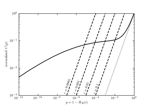
Illustration of the Benjamini and Hochberg method for 106 points drawn from the distribution shown in figure 4.5. The solid line shows the cumulative distribution of observed p values, normalized by the sample size. The dashed lines show the cutoff for various limits on contamination rate computed using eq. 4.44 (the accepted measurements are those with p smaller than that corresponding to the intersection of solid and dashed curves). The dotted line shows how the distribution would look in the absence of sources. The value of the cumulative distribution at p = 0.5 is 0.55, and yields a correction factor (see eq. 4.46).

Code output:

Python source code:

# Author: Jake VanderPlas
# License: BSD
#   The figure produced by this code is published in the textbook
#   "Statistics, Data Mining, and Machine Learning in Astronomy" (2013)
#   For more information, see http://astroML.github.com
#   To report a bug or issue, use the following forum:
#    https://groups.google.com/forum/#!forum/astroml-general
import numpy as np
from scipy.stats import norm
from matplotlib import pyplot as plt

#----------------------------------------------------------------------
# This function adjusts matplotlib settings for a uniform feel in the textbook.
# Note that with usetex=True, fonts are rendered with LaTeX.  This may
# result in an error if LaTeX is not installed on your system.  In that case,
# you can set usetex to False.
if "setup_text_plots" not in globals():
    from astroML.plotting import setup_text_plots
setup_text_plots(fontsize=8, usetex=True)

#------------------------------------------------------------
# Set up the background and foreground distributions
background = norm(100, 10)
foreground = norm(150, 12)
f = 0.1

# Draw from the distribution
np.random.seed(42)
N = int(1E6)
X = np.random.random(N)
mask = (X < 0.1)
X[mask] = foreground.rvs(np.sum(mask))
X[~mask] = background.rvs(np.sum(~mask))

#------------------------------------------------------------
# Perform Benjamini-Hochberg method
p = 1 - background.cdf(X)
p_sorted = np.sort(p)

#------------------------------------------------------------
# plot the results
fig = plt.figure(figsize=(5, 3.75))
fig.subplots_adjust(bottom=0.15)
ax = plt.axes(xscale='log', yscale='log')

# only plot every 1000th; plotting all 1E6 takes too long
ax.plot(p_sorted[::1000], np.linspace(0, 1, 1000), '-k')
ax.plot(p_sorted[::1000], p_sorted[::1000], ':k', lw=1)

# plot the cutoffs for various values of expsilon
p_reg_over_eps = 10 ** np.linspace(-3, 0, 100)
for (i, epsilon) in enumerate([0.1, 0.01, 0.001, 0.0001]):
    x = p_reg_over_eps * epsilon
    y = p_reg_over_eps
    ax.plot(x, y, '--k')

    ax.text(x[1], y[1],
            r'$\epsilon = %.1g$' % epsilon,
            ha='center', va='bottom', rotation=70)

ax.xaxis.set_major_locator(plt.LogLocator(base=100))

ax.set_xlim(1E-12, 1)
ax.set_ylim(1E-3, 1)

ax.set_xlabel('$p = 1 - H_B(i)$')
ax.set_ylabel('normalized $C(p)$')

plt.show()

[download source: fig_benjamini_method.py]