Example of classification
Figure 4.5.
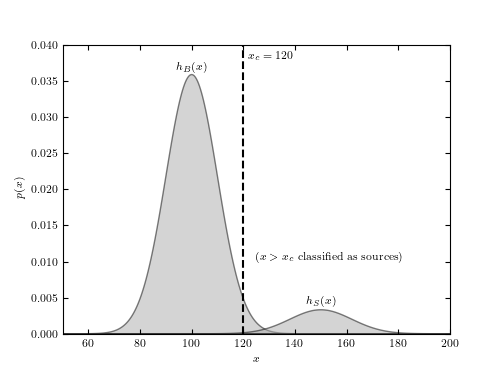
An example of a simple classification problem between two Gaussian
distributions. Given a value of x, we need to assign that measurement to one
of the two distributions (background vs. source). The cut at xc = 120 leads
to very few Type II errors (i.e., false negatives: points from the distribution
hS with x < xc being classified as background), but this comes at the cost of
a significant number of Type I errors (i.e., false positives: points from the
distribution  with x > xc being classified as sources).
# Author: Jake VanderPlas
# License: BSD
#   The figure produced by this code is published in the textbook
#   "Statistics, Data Mining, and Machine Learning in Astronomy" (2013)
#   For more information, see http://astroML.github.com
#   To report a bug or issue, use the following forum:
#    https://groups.google.com/forum/#!forum/astroml-general
import numpy as np
from scipy.stats import norm
from matplotlib import pyplot as plt

#----------------------------------------------------------------------
# This function adjusts matplotlib settings for a uniform feel in the textbook.
# Note that with usetex=True, fonts are rendered with LaTeX.  This may
# result in an error if LaTeX is not installed on your system.  In that case,
# you can set usetex to False.
if "setup_text_plots" not in globals():
    from astroML.plotting import setup_text_plots
setup_text_plots(fontsize=8, usetex=True)

#------------------------------------------------------------
# Generate and draw the curves
x = np.linspace(50, 200, 1000)
p1 = 0.9 * norm(100, 10).pdf(x)
p2 = 0.1 * norm(150, 12).pdf(x)

fig, ax = plt.subplots(figsize=(5, 3.75))
ax.fill(x, p1, ec='k', fc='#AAAAAA', alpha=0.5)
ax.fill(x, p2, '-k', fc='#AAAAAA', alpha=0.5)

ax.plot([120, 120], [0.0, 0.04], '--k')

ax.text(100, 0.036, r'$h_B(x)$', ha='center', va='bottom')
ax.text(150, 0.0035, r'$h_S(x)$', ha='center', va='bottom')
ax.text(122, 0.039, r'$x_c=120$', ha='left', va='top')
ax.text(125, 0.01, r'$(x > x_c\ {\rm classified\ as\ sources})$')

ax.set_xlim(50, 200)
ax.set_ylim(0, 0.04)

ax.set_xlabel('$x$')
ax.set_ylabel('$p(x)$')
plt.show()