Gaussianity Tests
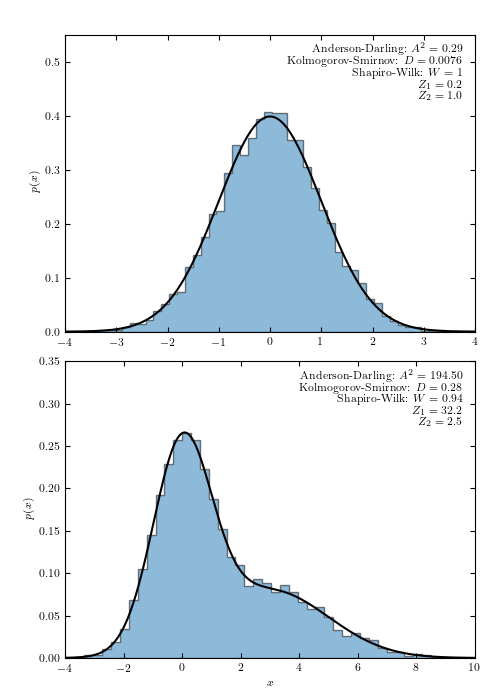
Figure 4.7.
The results of the Anderson-Darling test, the Kolmogorov-Smirnov test, and the Shapiro-Wilk test when applied to a sample of 10,000 values drawn from a normal distribution (upper panel) and from a combination of two Gaussian distributions (lower panel).
The functions are available in the scipy package:
The Anderson-Darling test (
scipy.stats.anderson)The Kolmogorov-Smirnov test (
scipy.stats.kstest)The Shapiro-Wilk test (
scipy.stats.shapiro)
______________________________________________________________________
  Kolmogorov-Smirnov test: D = 0.0076  p = 0.6
  Anderson-Darling test: A^2 = 0.29
    significance  | critical value
    --------------|----------------
    0.58          | 15.0%
    0.66          | 10.0%
    0.79          | 5.0%
    0.92          | 2.5%
    1.09          | 1.0%
  Shapiro-Wilk test: W = 1 p = 0.59
  Z_1 = 0.2
  Z_2 = 1.0
______________________________________________________________________
  Kolmogorov-Smirnov test: D = 0.28  p = 0
  Anderson-Darling test: A^2 = 1.9e+02
    significance  | critical value
    --------------|----------------
    0.58          | 15.0%
    0.66          | 10.0%
    0.79          | 5.0%
    0.92          | 2.5%
    1.09          | 1.0%
  Shapiro-Wilk test: W = 0.94 p = 0
  Z_1 = 32.2
  Z_2 = 2.5
# Author: Jake VanderPlas
# License: BSD
#   The figure produced by this code is published in the textbook
#   "Statistics, Data Mining, and Machine Learning in Astronomy" (2013)
#   For more information, see http://astroML.github.com
#   To report a bug or issue, use the following forum:
#    https://groups.google.com/forum/#!forum/astroml-general
from __future__ import print_function, division

import numpy as np
from scipy import stats
from matplotlib import pyplot as plt

#----------------------------------------------------------------------
# This function adjusts matplotlib settings for a uniform feel in the textbook.
# Note that with usetex=True, fonts are rendered with LaTeX.  This may
# result in an error if LaTeX is not installed on your system.  In that case,
# you can set usetex to False.
if "setup_text_plots" not in globals():
    from astroML.plotting import setup_text_plots
setup_text_plots(fontsize=8, usetex=True)

from astroML.stats import mean_sigma, median_sigmaG

# create some distributions
np.random.seed(1)
normal_vals = stats.norm(loc=0, scale=1).rvs(10000)
dual_vals = stats.norm(0, 1).rvs(10000)
dual_vals[:4000] = stats.norm(loc=3, scale=2).rvs(4000)

x = np.linspace(-4, 10, 1000)
normal_pdf = stats.norm(0, 1).pdf(x)
dual_pdf = 0.6 * stats.norm(0, 1).pdf(x) + 0.4 * stats.norm(3, 2).pdf(x)

vals = [normal_vals, dual_vals]
pdf = [normal_pdf, dual_pdf]
xlims = [(-4, 4), (-4, 10)]


#------------------------------------------------------------
# Compute the statistics and plot the results
fig = plt.figure(figsize=(5, 7))
fig.subplots_adjust(left=0.13, right=0.95,
                    bottom=0.06, top=0.95,
                    hspace=0.1)

for i in range(2):
    ax = fig.add_subplot(2, 1, 1 + i)  # 2 x 1 subplot

    # compute some statistics
    A2, sig, crit = stats.anderson(vals[i])
    D, pD = stats.kstest(vals[i], "norm")
    W, pW = stats.shapiro(vals[i])

    mu, sigma = mean_sigma(vals[i], ddof=1)
    median, sigmaG = median_sigmaG(vals[i])

    N = len(vals[i])
    Z1 = 1.3 * abs(mu - median) / sigma * np.sqrt(N)
    Z2 = 1.1 * abs(sigma / sigmaG - 1) * np.sqrt(N)

    print(70 * '_')
    print("  Kolmogorov-Smirnov test: D = %.2g  p = %.2g" % (D, pD))
    print("  Anderson-Darling test: A^2 = %.2g" % A2)
    print("    significance  | critical value ")
    print("    --------------|----------------")
    for j in range(len(sig)):
        print("    {0:.2f}          | {1:.1f}%".format(sig[j], crit[j]))
    print("  Shapiro-Wilk test: W = %.2g p = %.2g" % (W, pW))
    print("  Z_1 = %.1f" % Z1)
    print("  Z_2 = %.1f" % Z2)

    # plot a histogram
    ax.hist(vals[i], bins=50, density=True, histtype='stepfilled', alpha=0.5)
    ax.plot(x, pdf[i], '-k')
    ax.set_xlim(xlims[i])

    # print information on the plot
    info = "Anderson-Darling: $A^2 = %.2f$\n" % A2
    info += "Kolmogorov-Smirnov: $D = %.2g$\n" % D
    info += "Shapiro-Wilk: $W = %.2g$\n" % W
    info += "$Z_1 = %.1f$\n$Z_2 = %.1f$" % (Z1, Z2)
    ax.text(0.97, 0.97, info,
            ha='right', va='top', transform=ax.transAxes)

    if i == 0:
        ax.set_ylim(0, 0.55)
    else:
        ax.set_ylim(0, 0.35)
        ax.set_xlabel('$x$')

    ax.set_ylabel('$p(x)$')

plt.show()