The effect of Sampling
Figure 10.14
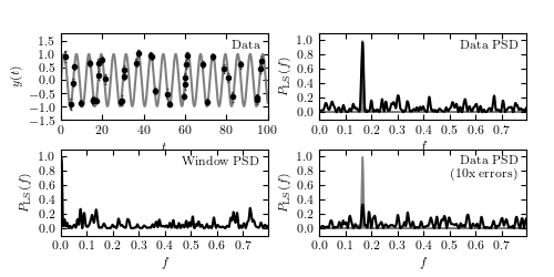
An illustration of the impact of measurement errors on the Lomb-Scargle power
(cf. figure 10.4). The top-left panel shows a simulated data set with 40 points
drawn from the function y(t|P) = sin(t) (i.e., f = 1/(2pi) ~ 0.16) with random
sampling. Heteroscedastic Gaussian noise is added to the observations, with a
width drawn from a uniform distribution with 0.1 < sigma < 0.2 (this error
level is negligible compared to the amplitude of variation). The spectral
window function (PSD of sampling times) is shown in the bottom-left panel.
The PSD ( ) computed for the data set from the top-left panel is
shown in the top-right panel; it is equal to a convolution of the single peak
(shaded in gray) with the window PSD shown in the bottom-left panel (e.g., the
peak at f ~ 0.42 in the top-right panel can be traced to a peak at f ~ 0.26 in
the bottom-left panel). The bottom-right panel shows the PSD for a data set
with errors increased by a factor of 10. Note that the peak f ~ 0.16 is now
much shorter, in agreement with eq. 10.47. In addition, errors now exceed the
amplitude of variation and the data PSD is no longer a simple convolution of
a single peak and the spectral window.
) computed for the data set from the top-left panel is
shown in the top-right panel; it is equal to a convolution of the single peak
(shaded in gray) with the window PSD shown in the bottom-left panel (e.g., the
peak at f ~ 0.42 in the top-right panel can be traced to a peak at f ~ 0.26 in
the bottom-left panel). The bottom-right panel shows the PSD for a data set
with errors increased by a factor of 10. Note that the peak f ~ 0.16 is now
much shorter, in agreement with eq. 10.47. In addition, errors now exceed the
amplitude of variation and the data PSD is no longer a simple convolution of
a single peak and the spectral window.
# Author: Jake VanderPlas
# License: BSD
#   The figure produced by this code is published in the textbook
#   "Statistics, Data Mining, and Machine Learning in Astronomy" (2013)
#   For more information, see http://astroML.github.com
#   To report a bug or issue, use the following forum:
#    https://groups.google.com/forum/#!forum/astroml-general
import numpy as np
import matplotlib
from matplotlib import pyplot as plt

from astroML.time_series import lomb_scargle

#----------------------------------------------------------------------
# This function adjusts matplotlib settings for a uniform feel in the textbook.
# Note that with usetex=True, fonts are rendered with LaTeX.  This may
# result in an error if LaTeX is not installed on your system.  In that case,
# you can set usetex to False.
if "setup_text_plots" not in globals():
    from astroML.plotting import setup_text_plots
setup_text_plots(fontsize=8, usetex=True)
matplotlib.rcParams['axes.xmargin'] = 0

#------------------------------------------------------------
# Generate the data
np.random.seed(42)
t_obs = 100 * np.random.random(40)  # 40 observations in 100 days
y_obs1 = np.sin(np.pi * t_obs / 3)
dy1 = 0.1 + 0.1 * np.random.random(y_obs1.shape)
y_obs1 += np.random.normal(0, dy1)

y_obs2 = np.sin(np.pi * t_obs / 3)
dy2 = 10 * dy1
y_obs2 = y_obs2 + np.random.normal(dy2)

y_window = np.ones_like(y_obs1)

t = np.linspace(0, 100, 10000)
y = np.sin(np.pi * t / 3)

#------------------------------------------------------------
# Compute the periodogram
omega = np.linspace(0, 5, 1001)[1:]
P_obs1 = lomb_scargle(t_obs, y_obs1, dy1, omega)
P_obs2 = lomb_scargle(t_obs, y_obs2, dy2, omega)
P_window = lomb_scargle(t_obs, y_window, 1, omega,
                        generalized=False, subtract_mean=False)
P_true = lomb_scargle(t, y, 1, omega)

omega /= 2 * np.pi

#------------------------------------------------------------
# Prepare the figures
fig = plt.figure(figsize=(5, 2.5))
fig.subplots_adjust(bottom=0.15, hspace=0.35, wspace=0.25,
                    left=0.11, right=0.95)

ax = fig.add_subplot(221)
ax.plot(t, y, '-', c='gray')
ax.errorbar(t_obs, y_obs1, dy1, fmt='.k', capsize=1, ecolor='#444444')
ax.text(0.96, 0.92, "Data", ha='right', va='top', transform=ax.transAxes)
ax.set_ylim(-1.5, 1.8)
ax.set_xlabel('$t$')
ax.set_ylabel('$y(t)$')

ax = fig.add_subplot(223)
ax.plot(omega, P_window, '-', c='black')
ax.text(0.96, 0.92, "Window PSD", ha='right', va='top', transform=ax.transAxes)
ax.set_ylim(-0.1, 1.1)
ax.set_xlabel('$f$')
ax.set_ylabel(r'$P_{\rm LS}(f)$')

ax = fig.add_subplot(222)
ax.fill(omega, P_true, fc='gray', ec='gray')
ax.plot(omega, P_obs1, '-', c='black')
ax.text(0.96, 0.92, "Data PSD", ha='right', va='top', transform=ax.transAxes)
ax.set_ylim(-0.1, 1.1)
ax.set_xlabel('$f$')
ax.set_ylabel(r'$P_{\rm LS}(f)$')

ax = fig.add_subplot(224)
ax.fill(omega, P_true, fc='gray', ec='gray')
ax.plot(omega, P_obs2, '-', c='black')
ax.text(0.96, 0.92, "Data PSD\n(10x errors)",
        ha='right', va='top', transform=ax.transAxes)
ax.set_ylim(-0.1, 1.1)
ax.set_xlabel('$f$')
ax.set_ylabel(r'$P_{\rm LS}(f)$')

plt.show()