Example of Minimum Component Filtering
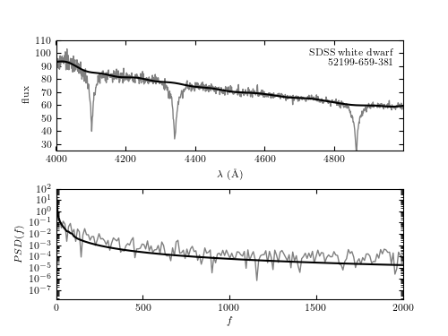
Figure 10.13
A minimum component filter applied to the spectrum of a white dwarf from SDSS data set (mjd= 52199, plate=659, fiber=381). The upper panel shows a portion of the input spectrum, along with the continuum computed via the minimum component filtering procedure described in Section 10.2.5 (see figure 10.12). The lower panel shows the PSD for both the input spectrum and the filtered result.
# Author: Jake VanderPlas
# License: BSD
#   The figure produced by this code is published in the textbook
#   "Statistics, Data Mining, and Machine Learning in Astronomy" (2013)
#   For more information, see http://astroML.github.com
#   To report a bug or issue, use the following forum:
#    https://groups.google.com/forum/#!forum/astroml-general
import numpy as np
from matplotlib import pyplot as plt

from astroML.fourier import PSD_continuous
from astroML.datasets import fetch_sdss_spectrum
from astroML.filters import min_component_filter

#----------------------------------------------------------------------
# This function adjusts matplotlib settings for a uniform feel in the textbook.
# Note that with usetex=True, fonts are rendered with LaTeX.  This may
# result in an error if LaTeX is not installed on your system.  In that case,
# you can set usetex to False.
if "setup_text_plots" not in globals():
    from astroML.plotting import setup_text_plots
setup_text_plots(fontsize=8, usetex=True)

#------------------------------------------------------------
# Fetch the spectrum from SDSS database & pre-process
plate = 659
mjd = 52199
fiber = 381

data = fetch_sdss_spectrum(plate, mjd, fiber)

lam = data.wavelength()
spec = data.spectrum

# wavelengths are logorithmically spaced: we'll work in log(lam)
loglam = np.log10(lam)

flag = (lam > 4000) & (lam < 5000)
lam = lam[flag]
loglam = loglam[flag]
spec = spec[flag]

lam = lam[:-1]
loglam = loglam[:-1]
spec = spec[:-1]

#----------------------------------------------------------------------
# Mask-out significant features and compute filtered version
feature_mask = (((lam > 4080) & (lam < 4130)) |
                ((lam > 4315) & (lam < 4370)) |
                ((lam > 4830) & (lam < 4900)))

spec_filtered = min_component_filter(loglam, spec, feature_mask, fcut=100)

#------------------------------------------------------------
# Compute PSD of filtered and unfiltered versions
f, spec_filt_PSD = PSD_continuous(loglam, spec_filtered)
f, spec_PSD = PSD_continuous(loglam, spec)

#------------------------------------------------------------
# Plot the results
fig = plt.figure(figsize=(5, 3.75))
fig.subplots_adjust(hspace=0.35)

# Top panel: plot noisy and smoothed spectrum
ax = fig.add_subplot(211)
ax.plot(lam, spec, '-', c='gray', lw=1)
ax.plot(lam, spec_filtered, '-k')

ax.text(0.97, 0.93, "SDSS white dwarf\n %i-%i-%i" % (mjd, plate, fiber),
        ha='right', va='top', transform=ax.transAxes)

ax.set_ylim(25, 110)

ax.set_xlabel(r'$\lambda\ {\rm (\AA)}$')
ax.set_ylabel('flux')

# Bottom panel: plot noisy and smoothed PSD
ax = fig.add_subplot(212, yscale='log')
ax.plot(f, spec_PSD, '-', c='gray', lw=1)
ax.plot(f, spec_filt_PSD, '-k')

ax.set_xlabel(r'$f$')
ax.set_ylabel('$PSD(f)$')
ax.set_xlim(0, 2000)

plt.show()