Matched Filter Chirp Search

Figure 10.27

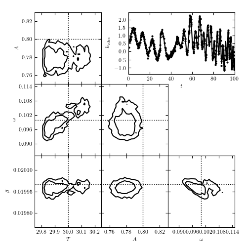
A ten-parameter chirp model (see eq. 10.87) fit to a time series. Seven of the parameters can be considered nuisance parameters, and we marginalize over them in the likelihood contours shown here.

Code output:

Python source code:

# Author: Jake VanderPlas (adapted to PyMC3 by Brigitta Sipocz)
# License: BSD
#   The figure produced by this code is published in the textbook
#   "Statistics, Data Mining, and Machine Learning in Astronomy" (2013)
#   For more information, see http://astroML.github.com
#   To report a bug or issue, use the following forum:
#    https://groups.google.com/forum/#!forum/astroml-general
import numpy as np
from matplotlib import pyplot as plt

import pymc3 as pm

from astroML.plotting.mcmc import plot_mcmc

# ----------------------------------------------------------------------
# This function adjusts matplotlib settings for a uniform feel in the textbook.
# Note that with usetex=True, fonts are rendered with LaTeX.  This may
# result in an error if LaTeX is not installed on your system.  In that case,
# you can set usetex to False.
if "setup_text_plots" not in globals():
    from astroML.plotting import setup_text_plots
setup_text_plots(fontsize=8, usetex=True)


# ----------------------------------------------------------------------
# Set up toy dataset
def chirp(t, T, A, phi, omega, beta):
    """chirp signal"""
    mask = (t >= T)
    signal = mask * (A * np.sin(phi + omega * (t - T) + beta * (t - T) ** 2))
    return signal


def background(t, b0, b1, omega1, omega2):
    """background signal"""
    return b0 + b1 * np.sin(omega1 * t) * np.sin(omega2 * t)


np.random.seed(0)
N = 500
T_true = 30
A_true = 0.8
phi_true = np.pi / 2
omega_true = 0.1
beta_true = 0.02
b0_true = 0.5
b1_true = 1.0
omega1_true = 0.3
omega2_true = 0.4
sigma = 0.1

t = 100 * np.random.random(N)

signal = chirp(t, T_true, A_true, phi_true, omega_true, beta_true)
bg = background(t, b0_true, b1_true, omega1_true, omega2_true)

y_true = signal + bg

y_obs = np.random.normal(y_true, sigma)

t_fit = np.linspace(0, 100, 1000)
y_fit = (chirp(t_fit, T_true, A_true, phi_true, omega_true, beta_true) +
         background(t_fit, b0_true, b1_true, omega1_true, omega2_true))


# ----------------------------------------------------------------------
# Set up and run MCMC sampling

with pm.Model():

    T = pm.Uniform('T', 0, 100, testval=T_true)
    A = pm.Uniform('A', 0, 100, testval=A_true)
    phi = pm.Uniform('phi', -np.pi, np.pi, testval=phi_true)

    b0 = pm.Uniform('b0', 0, 100, testval=b0_true)
    b1 = pm.Uniform('b1', 0, 100, testval=b1_true)

    log_omega1 = pm.Uniform('log_omega1', -3, 0, testval=np.log(omega1_true))
    log_omega2 = pm.Uniform('log_omega2', -3, 0, testval=np.log(omega2_true))

    omega = pm.Uniform('omega', 0.001, 1, testval=omega_true)
    beta = pm.Uniform('beta', 0.001, 1, testval=beta_true)

    y = pm.Normal('y', mu=(chirp(t, T, A, phi, omega, beta)
                           + background(t, b0, b1, np.exp(log_omega1), np.exp(log_omega2))),
                  tau=sigma ** -2, observed=y_obs)

    step = pm.Metropolis()

    traces = pm.sample(draws=5000, tune=2000, step=step)


labels = ['$T$', '$A$', r'$\omega$', r'$\beta$']
limits = [(29.75, 30.25), (0.75, 0.83), (0.085, 0.115), (0.0197, 0.0202)]
true = [T_true, A_true, omega_true, beta_true]

# ------------------------------------------------------------
# Plot results
fig = plt.figure(figsize=(5, 5))

# This function plots multiple panels with the traces
axes_list = plot_mcmc([traces[i] for i in ['T', 'A', 'omega', 'beta']],
                      labels=labels, limits=limits,
                      true_values=true, fig=fig,
                      bins=30, colors='k',
                      bounds=[0.14, 0.08, 0.95, 0.95])

for ax in axes_list:
    for axis in [ax.xaxis, ax.yaxis]:
        axis.set_major_locator(plt.MaxNLocator(5))

ax = fig.add_axes([0.52, 0.7, 0.43, 0.25])
ax.scatter(t, y_obs, s=9, lw=0, c='k')
ax.plot(t_fit, y_fit, '-k')
ax.set_xlim(0, 100)
ax.set_xlabel('$t$')
ax.set_ylabel(r'$h_{\rm obs}$')

plt.show()

[download source: fig_matchedfilt_chirp2.py]