Matched Filter Chirp Search

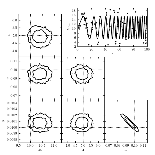
Figure 10.26

A matched filter search for a chirp signal in time series data. A simulated data set generated from a model of the form y = b0+Asin[omega t + beta t^2], with homoscedastic Gaussian errors with sigma = 2, is shown in the top-right panel. The posterior pdf for the four model parameters is determined using MCMC and shown in the other panels.

Code output:

Python source code:

# Author: Jake VanderPlas (adapted to PyMC3 by Brigitta Sipocz)
# License: BSD
#   The figure produced by this code is published in the textbook
#   "Statistics, Data Mining, and Machine Learning in Astronomy" (2013)
#   For more information, see http://astroML.github.com
#   To report a bug or issue, use the following forum:
#    https://groups.google.com/forum/#!forum/astroml-general
import numpy as np
from matplotlib import pyplot as plt

import pymc3 as pm

from astroML.plotting.mcmc import plot_mcmc

# ----------------------------------------------------------------------
# This function adjusts matplotlib settings for a uniform feel in the textbook.
# Note that with usetex=True, fonts are rendered with LaTeX.  This may
# result in an error if LaTeX is not installed on your system.  In that case,
# you can set usetex to False.
if "setup_text_plots" not in globals():
    from astroML.plotting import setup_text_plots

setup_text_plots(fontsize=8, usetex=True)


# ----------------------------------------------------------------------
# Set up toy dataset
def chirp(t, b0, beta, A, omega):
    return b0 + A * np.sin(omega * t + beta * t * t)


np.random.seed(0)

N = 100
b0_true = 10
A_true = 5
beta_true = 0.01
omega_true = 0.1
sigma = 2.0

t = 100 * np.random.random(N)

y_true = chirp(t, b0_true, beta_true, A_true, omega_true)
y_obs = np.random.normal(y_true, sigma)


# ----------------------------------------------------------------------
# Set up MCMC sampling
with pm.Model():
    b0 = pm.Uniform('b0', 0, 50, testval=50 * np.random.random())
    A = pm.Uniform('A', 0, 50, testval=50 * np.random.random())
    log_beta = pm.Uniform('log_beta', -10, 10, testval=-4.6)
    log_omega = pm.Uniform('log_omega', -10, 10, testval=-2.3)

    y = pm.Normal('y', mu=chirp(t, b0, np.exp(log_beta), A, np.exp(log_omega)),
                  sd=sigma, observed=y_obs)

    # Choose the Metropolis-Hastings step rather than rely on the default
    step = pm.Metropolis()
    traces = pm.sample(draws=5000, tune=2000, step=step)


# ----------------------------------------------------------------------
# Use the summary() function to provide statistics for each variable
mean_vals = pm.summary(traces)['mean']
mean_vals['omega'] = np.exp(mean_vals.pop('log_omega'))
mean_vals['beta'] = np.exp(mean_vals.pop('log_beta'))

labels = ['$b_0$', '$A$', r'$\omega$', r'$\beta$']
limits = [(9.5, 11.3), (3.6, 6.4), (0.065, 0.115), (0.00975, 0.01045)]
true = [b0_true, A_true, omega_true, beta_true]

fig = plt.figure(figsize=(5, 5))
ax = plt.axes([0.5, 0.7, 0.45, 0.25])

t_fit = np.linspace(0, 100, 1001)
y_fit = chirp(t_fit, **mean_vals)


# ----------------------------------------------------------------------
# Plot multiple panels with the traces
plt.scatter(t, y_obs, s=9, lw=0, c='k')
plt.plot(t_fit, y_fit, '-k')
plt.xlim(0, 100)
plt.xlabel('$t$')
plt.ylabel(r'$h_{\rm obs}$')

plot_mcmc([traces[ii] for ii in ['b0', 'A']]
          + [np.exp(traces['log_omega']), np.exp(traces['log_beta'])],
          labels=labels, limits=limits, true_values=true, fig=fig,
          bins=30, bounds=[0.12, 0.08, 0.95, 0.91], colors='k')
plt.show()

[download source: fig_matchedfilt_chirp.py]