Lomb-Scargle Aliasing

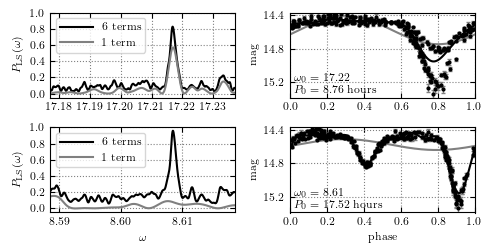
Figure 10.18

Analysis of a light curve where the standard Lomb-Scargle periodogram fails to find the correct period (the same star as in the top-left panel in figure 10.17). The two top panels show the periodograms (left) and phased light curves (right) for the truncated Fourier series model with M = 1 and M = 6 terms. Phased light curves are computed using the incorrect aliased period favored by the M = 1 model. The correct period is favored by the M = 6 model but unrecognized by the M = 1 model (bottom-left panel). The phased light curve constructed with the correct period is shown in the bottom-right panel. This case demonstrates that the Lomb-Scargle periodogram may easily fail when the signal shape significantly differs from a single sinusoid.

Code output:

Python source code:

# Author: Jake VanderPlas
# License: BSD
#   The figure produced by this code is published in the textbook
#   "Statistics, Data Mining, and Machine Learning in Astronomy" (2013)
#   For more information, see http://astroML.github.com
#   To report a bug or issue, use the following forum:
#    https://groups.google.com/forum/#!forum/astroml-general
import numpy as np
import matplotlib
from matplotlib import pyplot as plt

from astroML.time_series import multiterm_periodogram, MultiTermFit
from astroML.datasets import fetch_LINEAR_sample

#----------------------------------------------------------------------
# This function adjusts matplotlib settings for a uniform feel in the textbook.
# Note that with usetex=True, fonts are rendered with LaTeX.  This may
# result in an error if LaTeX is not installed on your system.  In that case,
# you can set usetex to False.
if "setup_text_plots" not in globals():
    from astroML.plotting import setup_text_plots
setup_text_plots(fontsize=8, usetex=True)
matplotlib.rcParams['axes.xmargin'] = 0

#------------------------------------------------------------
# Get data
data = fetch_LINEAR_sample()
t, y, dy = data[14752041].T

#------------------------------------------------------------
# Do a single-term and multi-term fit around the peak
omega0 = 17.217
nterms_fit = 6

# hack to get better phases: this doesn't change results,
#  except for how the phase plots are displayed
t -= 0.4 * np.pi / omega0

width = 0.03
omega = np.linspace(omega0 - width - 0.01, omega0 + width - 0.01, 1000)

#------------------------------------------------------------
# Compute periodograms and best-fit solutions
#  factor gives the factor that we're dividing the fundamental frequency by
factors = [1, 2]
nterms = [1, 6]

# Compute PSDs for factors & nterms
PSDs = dict()
for f in factors:
    for n in nterms:
        PSDs[(f, n)] = multiterm_periodogram(t, y, dy, omega / f, n)

# Compute the best-fit omega from the 6-term fit
omega_best = dict()
for f in factors:
    omegaf = omega / f
    PSDf = PSDs[(f, 6)]
    omega_best[f] = omegaf[np.argmax(PSDf)]

# Compute the best-fit solution based on the fundamental frequency
best_fit = dict()
for f in factors:
    for n in nterms:
        mtf = MultiTermFit(omega_best[f], n)
        mtf.fit(t, y, dy)
        phase_best, y_best = mtf.predict(1000, adjust_offset=False)

        best_fit[(f, n)] = (phase_best, y_best)

#------------------------------------------------------------
# Plot the results
fig = plt.figure(figsize=(5, 2.5))
fig.subplots_adjust(left=0.1, right=0.95, wspace=0.3,
                    bottom=0.15, top=0.95, hspace=0.35)

for i, f in enumerate(factors):
    P_best = 2 * np.pi / omega_best[f]
    phase_best = (t / P_best) % 1

    # first column: plot the PSD
    ax1 = fig.add_subplot(221 + 2 * i)
    ax1.plot(omega / f, PSDs[(f, 6)], '-', c='black', label='6 terms')
    ax1.plot(omega / f, PSDs[(f, 1)], '-', c='gray', label='1 term')
    ax1.grid(color='gray')
    ax1.legend(loc=2)

    ax1.axis('tight')

    ax1.set_ylim(-0.05, 1.001)
    ax1.xaxis.set_major_locator(plt.MultipleLocator(0.01))
    ax1.xaxis.set_major_formatter(plt.FormatStrFormatter('%.2f'))

    # second column: plot the phased data & fit
    ax2 = fig.add_subplot(222 + 2 * i)
    ax2.errorbar(phase_best, y, dy, fmt='.k', ms=4, ecolor='gray', lw=1,
                 capsize=1.5)
    ax2.plot(best_fit[(f, 1)][0], best_fit[(f, 1)][1], '-', c='gray')
    ax2.plot(best_fit[(f, 6)][0], best_fit[(f, 6)][1], '-', c='black')

    ax2.text(0.02, 0.02, (r"$\omega_0 = %.2f$" % omega_best[f] + "\n"
                          + r"$P_0 = %.2f\ {\rm hours}$" % (24 * P_best)),
             ha='left', va='bottom', transform=ax2.transAxes)

    ax2.grid(color='gray')
    ax2.set_xlim(0, 1)
    ax2.set_ylim(plt.ylim()[::-1])
    ax2.yaxis.set_major_locator(plt.MultipleLocator(0.4))

    # label both axes
    ax1.set_ylabel(r'$P_{\rm LS}(\omega)$')
    ax2.set_ylabel(r'${\rm mag}$')
    if i == 1:
        ax1.set_xlabel(r'$\omega$')
        ax2.set_xlabel(r'${\rm phase}$')

plt.show()

[download source: fig_LS_double_eclipse.py]