Measurement Errors in Linear Regression

Lets use simulated data here.

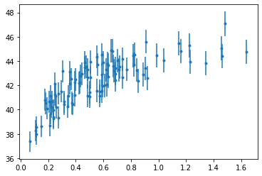
First we will model the distance of 100 supernovae (for a particular cosmology) as a function of redshift.

We rely on that astroML has a common API with scikit-learn, extending the functionality of the latter.

%matplotlib inline

import numpy as np
from matplotlib import pyplot as plt

from astropy.cosmology import LambdaCDM
from astroML.datasets import generate_mu_z

z_sample, mu_sample, dmu = generate_mu_z(100, random_state=0)

cosmo = LambdaCDM(H0=70, Om0=0.30, Ode0=0.70, Tcmb0=0)
z = np.linspace(0.01, 2, 1000)
mu_true = cosmo.distmod(z)

plt.errorbar(z_sample, mu_sample, dmu, fmt='.')

<ErrorbarContainer object of 3 artists>

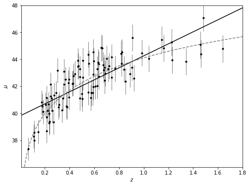
Simple linear regression

Regression defined as the relation between a dependent variable, \(y\), and a set of independent variables, \(x\), that describes the expectation value of y given x: \( E[y|x] \)

We will start with the most familiar linear regression, a straight-line fit to data. A straight-line fit is a model of the form $\( y = ax + b \)\( where \)a\( is commonly known as the *slope*, and \)b$ is commonly known as the intercept.

We can use Scikit-Learn’s LinearRegression estimator to fit this data and construct the best-fit line:

from sklearn.linear_model import LinearRegression as LinearRegression_sk 

linear_sk = LinearRegression_sk()
linear_sk.fit(z_sample[:,None], mu_sample)

mu_fit_sk = linear_sk.predict(z[:, None])

#------------------------------------------------------------
# Plot the results
fig = plt.figure(figsize=(8, 6))

ax = fig.add_subplot(111)

ax.plot(z, mu_fit_sk, '-k')
ax.plot(z, mu_true, '--', c='gray')
ax.errorbar(z_sample, mu_sample, dmu, fmt='.k', ecolor='gray', lw=1)

ax.set_xlim(0.01, 1.8)
ax.set_ylim(36.01, 48)

ax.set_ylabel(r'$\mu$')
ax.set_xlabel(r'$z$')

plt.show()

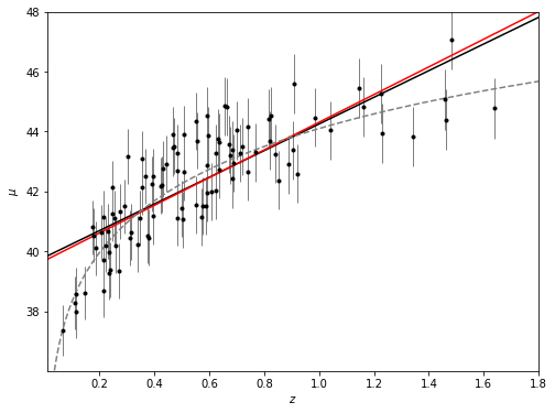
Measurement errors

Modifications to LinearRegression in astroML take measurement errors into account on the dependent variable.

from astroML.linear_model import LinearRegression

linear = LinearRegression()
linear.fit(z_sample[:,None], mu_sample, dmu)

mu_fit = linear.predict(z[:, None])

#------------------------------------------------------------
# Plot the results
fig = plt.figure(figsize=(8, 6))

ax = fig.add_subplot(111)

ax.plot(z, mu_fit_sk, '-k')
ax.plot(z, mu_fit, '-k', color='red')

ax.plot(z, mu_true, '--', c='gray')
ax.errorbar(z_sample, mu_sample, dmu, fmt='.k', ecolor='gray', lw=1)

ax.set_xlim(0.01, 1.8)
ax.set_ylim(36.01, 48)

ax.set_ylabel(r'$\mu$')
ax.set_xlabel(r'$z$')

plt.show()

Basis function regression

If we consider a function in terms of the sum of bases (this can be polynomials, Gaussians, quadratics, cubics) then we can solve for the coefficients using regression.

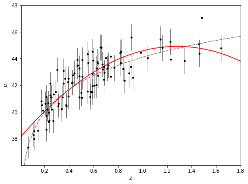
Polynomial basis functions

polynomial regression:

\[y=a_0+a_1x+a_2x^2+a_3x^3+...\]

Notice that this is still a linear model—the linearity refers to the fact that the coefficients \(a_n\) never multiply or divide each other. What we have effectively done here is to take our one-dimensional \(x\) values and projected them into a higher dimension, so that a linear fit can fit more complicated relationships between \(x\) and \(y\).

from astroML.linear_model import PolynomialRegression

# 2nd degree polynomial regression
polynomial = PolynomialRegression(degree=2)
polynomial.fit(z_sample[:,None], mu_sample, dmu)

mu_fit_poly = polynomial.predict(z[:, None])

#------------------------------------------------------------
# Plot the results
fig = plt.figure(figsize=(8, 6))

ax = fig.add_subplot(111)

ax.plot(z, mu_fit_poly, '-k', color='red')

ax.plot(z, mu_true, '--', c='gray')
ax.errorbar(z_sample, mu_sample, dmu, fmt='.k', ecolor='gray', lw=1)

ax.set_xlim(0.01, 1.8)
ax.set_ylim(36.01, 48)

ax.set_ylabel(r'$\mu$')
ax.set_xlabel(r'$z$')

plt.show()

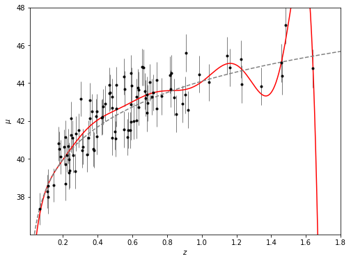
Gaussian basis functions

Of course, other basis functions are possible. For example, one useful pattern is to fit a model that is not a sum of polynomial bases, but a sum of Gaussian bases. E.g. we could substitute \(x^2\) for Gaussians (where we fix \(\sigma\) and \(\mu\) and fit for the amplitude) as long as the attribute we are fitting for is linear. This is called basis function regression.

from astroML.linear_model import BasisFunctionRegression

#------------------------------------------------------------
# Define our number of Gaussians
nGaussians = 10
basis_mu = np.linspace(0, 2, nGaussians)[:, None]
basis_sigma = 3 * (basis_mu[1] - basis_mu[0])

gauss_basis = BasisFunctionRegression('gaussian', mu=basis_mu, sigma=basis_sigma)
gauss_basis.fit(z_sample[:,None], mu_sample, dmu)

mu_fit_gauss = gauss_basis.predict(z[:, None])

#------------------------------------------------------------
# Plot the results
fig = plt.figure(figsize=(8, 6))

ax = fig.add_subplot(111)

ax.plot(z, mu_fit_gauss, '-k', color='red')

ax.plot(z, mu_true, '--', c='gray')
ax.errorbar(z_sample, mu_sample, dmu, fmt='.k', ecolor='gray', lw=1)

ax.set_xlim(0.01, 1.8)
ax.set_ylim(36.01, 48)

ax.set_ylabel(r'$\mu$')
ax.set_xlabel(r'$z$')

plt.show()