Sesar 2010 RR Lyrae (Stripe 82)
The primary dataset available is the 483 RR Lyrae from Sesar 2010. This dataset contains observations of 483 RR Lyrae stars in Stripe 82 over approximately a decade, along with observational metadata, derived metadata, and templates derived from the code.
Observed Light Curves
The photometric light curves for these stars can be downloaded and accessed
via the fetch_rrlyrae() function. For example:
In [1]: from gatspy.datasets import fetch_rrlyrae

In [2]: rrlyrae = fetch_rrlyrae()

In [3]: len(rrlyrae.ids)
Out[3]: 483
As you can see, the result of the download is an object which contains the data
for all 483 lightcurves. You can fetch an individual lightcurve using the
get_lightcurve method, which takes a lightcurve id as an argument:
In [4]: lcid = rrlyrae.ids[0]

In [5]: t, mag, dmag, filts = rrlyrae.get_lightcurve(lcid)
Let’s use matplotlib to visualize this data, and get a feel for what is there:
(Source code, png, hires.png, pdf)
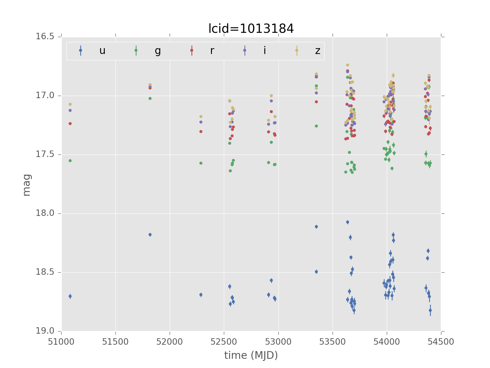
This gives a nice visual indication of what the data look like.
RR Lyrae Metadata
Along with the main lightcurve observations, the dataset tools give access to
two sets of metadata associated with the lightcurves. There is the observational
metadata available from the get_obsmeta() method, and the fit metadata
available in the get_metadata() method.
The observational metadata includes quantities like RA, Dec, extinction, etc. Details are in Table 3 of Sesar (2010).
In [6]: obsmeta = rrlyrae.get_obsmeta(lcid)

In [7]: print(obsmeta.dtype.names)
('id', 'RA', 'DEC', 'rExt', 'd', 'RGC', 'u', 'g', 'r', 'i', 'z', 'V', 'ugmin', 'ugmin_err', 'grmin', 'grmin_err')
The fit metadata includes quantities like the period, type of RR Lyrae, etc. Details are in Table 2 of Sesar (2010).
In [8]: metadata = rrlyrae.get_metadata(lcid)

In [9]: print(metadata.dtype.names)
('id', 'type', 'P', 'uA', 'u0', 'uE', 'uT', 'gA', 'g0', 'gE', 'gT', 'rA', 'r0', 'rE', 'rT', 'iA', 'i0', 'iE', 'iT', 'zA', 'z0', 'zE', 'zT')
For example, we can use the period from the metadata to phase the lightcurve as follows:
In [10]: period = metadata['P']

In [11]: phase = (t / period) % 1
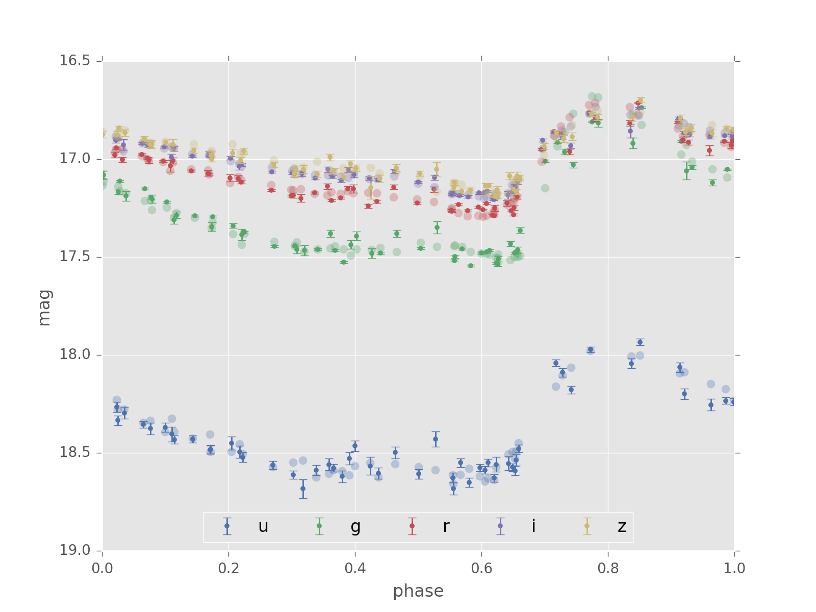
Using this, we can plot the phased lightcurve, which lets us more easily see the structure across the observations:
(Source code, png, hires.png, pdf)
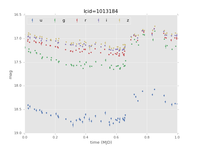
These periods were determined within Sesar 2010 via a template fitting approach.
RR Lyrae Templates
gatspy also provides a loader for the empirical RR Lyrae templates derived
in Sesar 2010. These are available via the
fetch_rrlyrae_templates() function:
In [12]: from gatspy.datasets import fetch_rrlyrae_templates

In [13]: templates = fetch_rrlyrae_templates()

In [14]: len(templates.ids)
Out[14]: 98
There are 98 templates spread among the five bands, which can be referenced by their id:
In [15]: templates.ids[:10]
Out[15]: ['0g', '0i', '0r', '0u', '0z', '100g', '100i', '100r', '100u', '100z']
Each of these templates is normalized from 0 to 1 in phase, and from 0 to 1 in
magnitude. For example, plotting template '100' we see:
(Source code, png, hires.png, pdf)
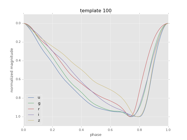
For more information on these templates, see the discussion in Sesar (2010).
Generated Lightcurves
Using the RR Lyrae templates, it is possible to simulate observations of RR
Lyrae stars. gatspy provides the RRLyraeGenerated
class as an interface for this.
In order to make the observations as realistic as possible, these lightcurves
are based on one of the 483 Stripe 82 RR Lyrae compiled by Sesar (2010):
In [16]: from gatspy.datasets import fetch_rrlyrae, RRLyraeGenerated

In [17]: rrlyrae = fetch_rrlyrae()

In [18]: lcid = rrlyrae.ids[0]

In [19]: gen = RRLyraeGenerated(lcid, random_state=0)

In [20]: mag = gen.generated('g', [51080.0, 51080.5], err=0.3)

In [21]: mag.round(2)
Out[21]: array([ 17.74,  17.04])
This will create observations drawn from the best-fit template with the given magnitude error. Here let’s use the observed times and errors to compare a realization of the generated light curve to the true observed data:
(Source code, png, hires.png, pdf)
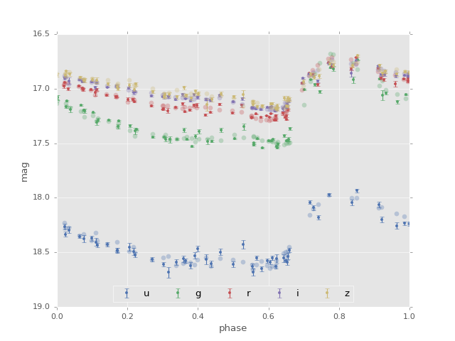
Here the observed data are the faint circles, while the generated data are the small points with errorbars. With this tool, it is easy to mimic observations of fainter RR Lyrae which follow the properties of the RR Lyrae observed in Stripe 82.