SVM Diagram
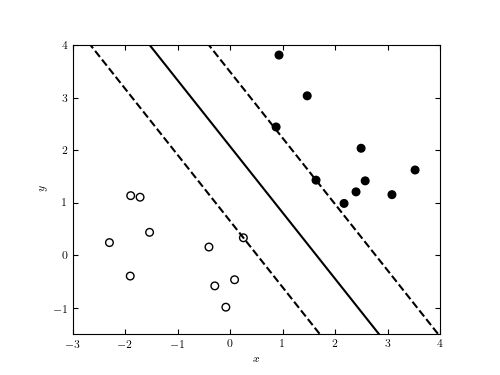
Figure 9.9
Illustration of SVM. The region between the dashed lines is the margin, and the points which the dashed lines touch are called the support vectors.
# Author: Jake VanderPlas
# License: BSD
#   The figure produced by this code is published in the textbook
#   "Statistics, Data Mining, and Machine Learning in Astronomy" (2013)
#   For more information, see http://astroML.github.com
#   To report a bug or issue, use the following forum:
#    https://groups.google.com/forum/#!forum/astroml-general
import numpy as np
from matplotlib import pyplot as plt
from sklearn import svm

#----------------------------------------------------------------------
# This function adjusts matplotlib settings for a uniform feel in the textbook.
# Note that with usetex=True, fonts are rendered with LaTeX.  This may
# result in an error if LaTeX is not installed on your system.  In that case,
# you can set usetex to False.
if "setup_text_plots" not in globals():
    from astroML.plotting import setup_text_plots
setup_text_plots(fontsize=8, usetex=True)

#------------------------------------------------------------
# Create the data
np.random.seed(1)

N1 = 10
N2 = 10
mu1 = np.array([0, 0])
mu2 = np.array([2.0, 2.0])

Cov1 = np.array([[1, -0.5],
                [-0.5, 1]])
Cov2 = Cov1

X = np.vstack([np.random.multivariate_normal(mu1, Cov1, N1),
               np.random.multivariate_normal(mu2, Cov2, N2)])
y = np.hstack([np.zeros(N1), np.ones(N2)])

#------------------------------------------------------------
# Perform an SVM classification
clf = svm.SVC(kernel='linear')
clf.fit(X, y)

xx = np.linspace(-5, 5)
w = clf.coef_[0]
m = -w[0] / w[1]
b = - clf.intercept_[0] / w[1]
yy = m * xx + b

#------------------------------------------------------------
# find support vectors
i1 = np.argmax(np.dot(X[:N1], w))
i2 = N1 + np.argmin(np.dot(X[N1:], w))

db1 = X[i1, 1] - (m * X[i1, 0] + b)
db2 = X[i2, 1] - (m * X[i2, 0] + b)

#------------------------------------------------------------
# Plot the results
fig = plt.figure(figsize=(5, 3.75))
ax = fig.add_subplot(111, aspect='equal')

ax.scatter(X[:, 0], X[:, 1], c=y, s=30, cmap=plt.cm.binary)
ax.plot(xx, yy, '-k')
ax.plot(xx, yy + db1, '--k')
ax.plot(xx, yy + db2, '--k')

ax.set_ylim(-1.5, 4)
ax.set_xlim(-3, 4)

ax.set_xlabel('$x$')
ax.set_ylabel('$y$')

plt.show()