# Author: Jake VanderPlas & Brigitta Sipocz
# License: BSD
# The figure produced by this code is published in the textbook
# "Statistics, Data Mining, and Machine Learning in Astronomy" (2019)
# For more information, see http://astroML.github.com
# To report a bug or issue, use the following forum:
# https://groups.google.com/forum/#!forum/astroml-general
import numpy as np
from matplotlib import pyplot as plt
#----------------------------------------------------------------------
# This function adjusts matplotlib settings for a uniform feel in the textbook.
# Note that with usetex=True, fonts are rendered with LaTeX. This may
# result in an error if LaTeX is not installed on your system. In that case,
# you can set usetex to False.
if "setup_text_plots" not in globals():
from astroML.plotting import setup_text_plots
setup_text_plots(fontsize=12, usetex=True)
fig = plt.figure(figsize=(6, 4), facecolor='w')
ax = fig.add_axes([0, 0, 1, 1],
xticks=[], yticks=[])
plt.box(False)
circ = plt.Circle((1, 1), 2)
radius = 0.3
# function to draw arrows
def draw_connecting_arrow(ax, circ1, rad1, circ2, rad2,
arrow_kwargs={'head_width': 0.05, 'fc': 'black'}):
theta = np.arctan2(circ2[1] - circ1[1],
circ2[0] - circ1[0])
starting_point = (circ1[0] + rad1 * np.cos(theta),
circ1[1] + rad1 * np.sin(theta))
length = (circ2[0] - circ1[0] - (rad1 + 1.4 * rad2) * np.cos(theta),
circ2[1] - circ1[1] - (rad1 + 1.4 * rad2) * np.sin(theta))
ax.arrow(starting_point[0], starting_point[1],
length[0], length[1], **arrow_kwargs)
# function to draw circles
def draw_circle(ax, center, radius):
circ = plt.Circle(center, radius, fc='none', lw=2)
ax.add_patch(circ)
x1 = -3
x2 = 0
x3 = 3
y3 = -0.75
# ------------------------------------------------------------
# draw circles
for i, y1 in enumerate(np.linspace(1.5, -2.5, 5)):
draw_circle(ax, (x1, y1), radius)
ax.text(x1 - 0.9, y1, '$x_{}$'.format(i + 1),
ha='right', va='center')
draw_connecting_arrow(ax, (x1 - 0.9, y1), 0.1, (x1, y1), radius)
for i, y2 in enumerate(np.linspace(1.25, -2.25, 4)):
draw_circle(ax, (x2, y2), radius)
ax.text(x2, y2, r'$f(\theta)$', fontsize=12, ha='center', va='center')
ax.text(x2 + radius * 0.9, y2 +radius, '$a_{}$'.format(i + 1), ha='center')
draw_circle(ax, (x3, y3), radius)
ax.text(x3 + 0.8, y3, '$o_k$', ha='left', va='center')
draw_connecting_arrow(ax, (x3, y3), radius, (x3 + 0.8, y3), 0.1)
ax.text(x3, y3, r'$g(\theta)$', fontsize=12, ha='center', va='center')
# ------------------------------------------------------------
# draw connecting arrows
for i, y1 in enumerate(np.linspace(1.5, -2.5, 5)):
for j, y2 in enumerate(np.linspace(1.25, -2.25, 4)):
# we only label a 2 sets of arrows to avoid overcrowding the figure
if i not in [0, 4]:
arrow_kwargs = {'head_width': 0.05, 'fc': 'black', 'alpha': 0.5}
else:
arrow_kwargs = {'head_width': 0.05, 'fc': 'black'}
draw_connecting_arrow(ax, (x1, y1), radius, (x2, y2), radius,
arrow_kwargs=arrow_kwargs)
if i % 5 == 0:
va = 'bottom'
shift = 0.1
else:
va = 'top'
shift = -0.1
if i in [0, 4]:
ax.text((2*x1+x2)/3, (2*y1+y2)/3 + shift,
'$w_{%s%s}$' % ((i+1), (j+1)), va=va, fontsize=12,
ha='center')
for i, y2 in enumerate(np.linspace(1.25, -2.25, 4)):
draw_connecting_arrow(ax, (x2, y2), radius, (x3, y3), radius)
ax.text((x2+x3)/2, (y2+y3)/2 + 0.1, '$w_{%sk}$' % (i+1),
fontsize=12, ha='center', va='bottom')
# ------------------------------------------------------------
# Add text labels
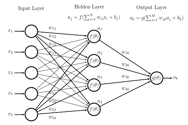
plt.text(x1, 2.7, "Input Layer", ha='center', va='top')
plt.text(x2, 2.7, r"Hidden Layer\\\\ $a_j=f(\sum_{i=1}^N w_{ij} x_i + b_j)$",
ha='center', va='top')
plt.text(x3, 2.7, r"Output Layer\\\\ $o_k=g(\sum_{j=1}^M w_{jk} a_j + b_k)$",
ha='center', va='top')
ax.set_aspect('equal')
plt.xlim(-4, 4)
plt.ylim(-3, 3)
plt.show()