Regularized Regression Example

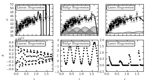
Figure 8.4

Regularized regression for the same sample as Fig. 8.2. Here we use Gaussian basis function regression with a Gaussian of width sigma = 0.2 centered at 100 regular intervals between 0 < z < 2. The lower panels show the best-fit weights as a function of basis function position. The left column shows the results with no regularization: the basis function weights w are on the order of 108, and overfitting is evident. The middle column shows ridge regression (L2 regularization) with alpha = 0.005, and the right column shows LASSO regression (L1 regularization) with alpha = 0.005. All three methods are fit without the bias term (intercept).

Changes from Published Version

Note that this figure has been changed slightly from its published version: the original version of the figure did not take into account data errors. The update (as of astroML version 0.3) correctly takes into account data errors.

Code output:

Python source code:

# Author: Jake VanderPlas
# License: BSD
#   The figure produced by this code is published in the textbook
#   "Statistics, Data Mining, and Machine Learning in Astronomy" (2013)
#   For more information, see http://astroML.github.com
#   To report a bug or issue, use the following forum:
#    https://groups.google.com/forum/#!forum/astroml-general
import numpy as np
from matplotlib import pyplot as plt

from astropy.cosmology import LambdaCDM

from astroML.linear_model import LinearRegression
from astroML.datasets import generate_mu_z

#----------------------------------------------------------------------
# This function adjusts matplotlib settings for a uniform feel in the textbook.
# Note that with usetex=True, fonts are rendered with LaTeX.  This may
# result in an error if LaTeX is not installed on your system.  In that case,
# you can set usetex to False.
if "setup_text_plots" not in globals():
    from astroML.plotting import setup_text_plots
setup_text_plots(fontsize=8, usetex=True)

#----------------------------------------------------------------------
# generate data
np.random.seed(0)

z_sample, mu_sample, dmu = generate_mu_z(100, random_state=0)
cosmo = LambdaCDM(H0=70, Om0=0.30, Ode0=0.70, Tcmb0=0)

z = np.linspace(0.01, 2, 1000)
mu = cosmo.distmod(z).value


#------------------------------------------------------------
# Manually convert data to a gaussian basis
#  note that we're ignoring errors here, for the sake of example.
def gaussian_basis(x, mu, sigma):
    return np.exp(-0.5 * ((x - mu) / sigma) ** 2)


centers = np.linspace(0, 1.8, 100)
widths = 0.2
X = gaussian_basis(z_sample[:, np.newaxis], centers, widths)

#------------------------------------------------------------
# Set up the figure to plot the results
fig = plt.figure(figsize=(5, 2.7))
fig.subplots_adjust(left=0.1, right=0.95,
                    bottom=0.12, top=0.95,
                    hspace=0.15, wspace=0.2)

regularization = ['none', 'l2', 'l1']
kwargs = [dict(), dict(alpha=0.005), dict(alpha=0.001)]
labels = ['Linear Regression', 'Ridge Regression', 'Lasso Regression']

for i in range(3):
    clf = LinearRegression(regularization=regularization[i],
                           fit_intercept=True, kwds=kwargs[i])
    clf.fit(X, mu_sample, dmu)
    w = clf.coef_[1:]
    fit = clf.predict(gaussian_basis(z[:, None], centers, widths))

    # plot fit
    ax = fig.add_subplot(231 + i)
    ax.xaxis.set_major_formatter(plt.NullFormatter())

    # plot curves for regularized fits
    if i == 0:
        ax.set_ylabel('$\mu$')
    else:
        ax.yaxis.set_major_formatter(plt.NullFormatter())
        curves = 37 + w * gaussian_basis(z[:, np.newaxis], centers, widths)
        curves = curves[:, abs(w) > 0.01]
        ax.plot(z, curves,
                c='gray', lw=1, alpha=0.5)

    ax.plot(z, fit, '-k')
    ax.plot(z, mu, '--', c='gray')
    ax.errorbar(z_sample, mu_sample, dmu, fmt='.k', ecolor='gray', lw=1, ms=4)
    ax.set_xlim(0.001, 1.8)
    ax.set_ylim(36, 52)
    ax.text(0.05, 0.93, labels[i],
            ha='left', va='top',
            bbox=dict(boxstyle='round', ec='k', fc='w'),
            transform=ax.transAxes)

    # plot weights
    ax = plt.subplot(234 + i)
    ax.xaxis.set_major_locator(plt.MultipleLocator(0.5))
    ax.set_xlabel('$z$')
    if i == 0:
        ax.set_ylabel(r'$\theta$')
        w *= 1E-12
        ax.text(0, 1.01, r'$\rm \times 10^{12}$',
                transform=ax.transAxes)
    ax.scatter(centers, w, s=9, lw=0, c='k')

    ax.set_xlim(-0.05, 1.8)

    if i == 1:
        ax.set_ylim(-2, 4)
    elif i == 2:
        ax.set_ylim(-0.5, 2)

    ax.text(0.05, 0.93, labels[i],
            ha='left', va='top',
            bbox=dict(boxstyle='round', ec='k', fc='w'),
            transform=ax.transAxes)

plt.show()

[download source: fig_rbf_ridge_mu_z.py]