Plot a visual representation of an SVD
Figure 7.3
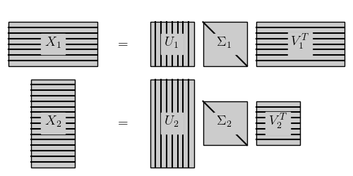
Singular value decomposition (SVD) can factorize an N x K matrix into
 . There are different conventions for computing the SVD
in the literature, and this figure illustrates the convention used in this
text. The matrix of singular values
. There are different conventions for computing the SVD
in the literature, and this figure illustrates the convention used in this
text. The matrix of singular values  is always a square matrix
of size [R x R] where R = min(N, K). The shape of the resulting U and V
matrices depends on whether N or K is larger. The columns of the matrix U are
called the left-singular vectors, and the columns of the matrix V are called
the right-singular vectors. The columns are orthonormal bases, and satisfy
is always a square matrix
of size [R x R] where R = min(N, K). The shape of the resulting U and V
matrices depends on whether N or K is larger. The columns of the matrix U are
called the left-singular vectors, and the columns of the matrix V are called
the right-singular vectors. The columns are orthonormal bases, and satisfy
 .
.
# Author: Jake VanderPlas
# License: BSD
#   The figure produced by this code is published in the textbook
#   "Statistics, Data Mining, and Machine Learning in Astronomy" (2013)
#   For more information, see http://astroML.github.com
#   To report a bug or issue, use the following forum:
#    https://groups.google.com/forum/#!forum/astroml-general
import numpy as np
from matplotlib import pyplot as plt
from matplotlib.patches import Rectangle

#----------------------------------------------------------------------
# This function adjusts matplotlib settings for a uniform feel in the textbook.
# Note that with usetex=True, fonts are rendered with LaTeX.  This may
# result in an error if LaTeX is not installed on your system.  In that case,
# you can set usetex to False.
if "setup_text_plots" not in globals():
    from astroML.plotting import setup_text_plots
setup_text_plots(fontsize=8, usetex=True)


# Define a function to create a rectangle
def labeled_rect(ax, center, width, height, text,
                 stripe='vert', N=7, color='#CCCCCC'):
    left = center[0] - 0.5 * width
    bottom = center[1] - 0.5 * height
    ax.add_patch(Rectangle((left, bottom), width, height,
                           fill=True, color=color, ec='k'))
    ax.text(center[0], center[1], text,
            fontsize=14, ha='center', va='center',
            bbox=dict(ec=color, fc=color))

    if stripe == 'vert':
        xlocs = np.linspace(center[0] - 0.5 * width,
                            center[0] + 0.5 * width,
                            N + 2)[1:-1]
        for x in xlocs:
            plt.plot([x, x],
                     [center[1] - 0.5 * height,
                      center[1] + 0.5 * height], '-k')

    elif stripe == 'horiz':
        ylocs = np.linspace(center[1] - 0.5 * height,
                            center[1] + 0.5 * height,
                            N + 2)[1:-1]
        for y in ylocs:
            plt.plot([center[0] - 0.5 * width,
                      center[0] + 0.5 * width],
                     [y, y], '-k')

    elif stripe == 'diag':
        plt.plot([center[0] - 0.5 * width, center[0] + 0.5 * width],
                 [center[1] + 0.5 * height, center[1] - 0.5 * height], '-k')
    else:
        raise ValueError("unrecognized stripe type")

#------------------------------------------------------------
# Plot the results
fig = plt.figure(figsize=(5, 2.5))
fig.subplots_adjust(left=0, bottom=0,
                    right=1, top=1)
ax = fig.add_subplot(111, xticks=[], yticks=[], frameon=False)

labeled_rect(ax, (0.3, 0.75), 0.5, 0.25, '$X_1$', 'horiz')
labeled_rect(ax, (0.975, 0.75), 0.25, 0.25, '$U_1$', 'vert')
labeled_rect(ax, (1.275, 0.75), 0.25, 0.25, r'$\Sigma_1$', 'diag')
labeled_rect(ax, (1.7, 0.75), 0.5, 0.25, r'$V_1^T$', 'horiz')

labeled_rect(ax, (0.3, 0.3), 0.25, 0.5, r'$X_2$', 'horiz', N=15)
labeled_rect(ax, (0.975, 0.3), 0.25, 0.5, r'$U_2$', 'vert')
labeled_rect(ax, (1.275, 0.3), 0.25, 0.25, r'$\Sigma_2$', 'diag')
labeled_rect(ax, (1.575, 0.3), 0.25, 0.25, r'$V_2^T$', 'horiz')

ax.text(0.7, 0.75, '$=$', fontsize=14, ha='center', va='center')
ax.text(0.7, 0.3, '$=$', fontsize=14, ha='center', va='center')

ax.set_xlim(0, 2)
ax.set_ylim(0, 1)

plt.show()