SDSS Eigenvalues

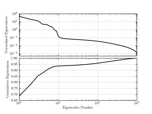
Figure 7.5

The eigenvalues for the PCA decomposition of the SDSS spectra described in Section 7.3.2. The top panel shows the decrease in eigenvalue as a function of the number of eigenvectors, with a break in the distribution at ten eigenvectors. The lower panel shows the cumulative sum of eigenvalues normalized to unity. 94% of the variance in the SDSS spectra can be captured using the first ten eigenvectors.

Code output:

Python source code:

# Author: Jake VanderPlas
# License: BSD
#   The figure produced by this code is published in the textbook
#   "Statistics, Data Mining, and Machine Learning in Astronomy" (2013)
#   For more information, see http://astroML.github.com
#   To report a bug or issue, use the following forum:
#    https://groups.google.com/forum/#!forum/astroml-general
import numpy as np
from matplotlib import pyplot as plt
from astroML import datasets

#----------------------------------------------------------------------
# This function adjusts matplotlib settings for a uniform feel in the textbook.
# Note that with usetex=True, fonts are rendered with LaTeX.  This may
# result in an error if LaTeX is not installed on your system.  In that case,
# you can set usetex to False.
if "setup_text_plots" not in globals():
    from astroML.plotting import setup_text_plots
setup_text_plots(fontsize=8, usetex=True)

#------------------------------------------------------------
# load data:
data = datasets.fetch_sdss_corrected_spectra()
spectra = datasets.sdss_corrected_spectra.reconstruct_spectra(data)

# Eigenvalues can be computed using PCA as in the commented code below:

#from sklearn.decomposition import PCA
#pca = PCA()
#pca.fit(spectra)
#evals = pca.explained_variance_ratio_
#evals_cs = evals.cumsum()

#  because the spectra have been reconstructed from masked values, this
#  is not exactly correct in this case: we'll use the values computed
#  in the file compute_sdss_pca.py
evals = data['evals'] ** 2
evals_cs = evals.cumsum()
evals_cs /= evals_cs[-1]

#------------------------------------------------------------
# plot the eigenvalues
fig = plt.figure(figsize=(5, 3.75))
fig.subplots_adjust(hspace=0.05, bottom=0.12)

ax = fig.add_subplot(211, xscale='log', yscale='log')
ax.grid()
ax.plot(evals, c='k')
ax.set_ylabel('Normalized Eigenvalues')
ax.xaxis.set_major_formatter(plt.NullFormatter())
ax.set_ylim(5E-4, 100)

ax = fig.add_subplot(212, xscale='log')
ax.grid()
ax.semilogx(evals_cs, color='k')
ax.set_xlabel('Eigenvalue Number')
ax.set_ylabel('Cumulative Eigenvalues')
ax.set_ylim(0.65, 1.00)

plt.show()

[download source: fig_eigenvalues.py]