Comparison of PCA and Manifold Learning

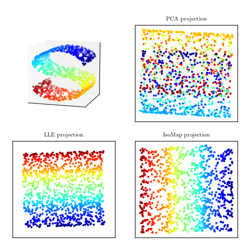
Figure 7.8

A comparison of PCA and manifold learning. The top-left panel shows an example S-shaped data set (a two-dimensional manifold in a three-dimensional space). PCA identifies three principal components within the data. Projection onto the first two PCA components results in a mixing of the colors along the manifold. Manifold learning (LLE and IsoMap) preserves the local structure when projecting the data, preventing the mixing of the colors.

Code output:

Python source code:

# Author: Jake VanderPlas
# License: BSD
#   The figure produced by this code is published in the textbook
#   "Statistics, Data Mining, and Machine Learning in Astronomy" (2013)
#   For more information, see http://astroML.github.com
#   To report a bug or issue, use the following forum:
#    https://groups.google.com/forum/#!forum/astroml-general
import numpy as np
from matplotlib import pyplot as plt
from matplotlib import ticker

from sklearn import manifold, datasets, decomposition

#----------------------------------------------------------------------
# This function adjusts matplotlib settings for a uniform feel in the textbook.
# Note that with usetex=True, fonts are rendered with LaTeX.  This may
# result in an error if LaTeX is not installed on your system.  In that case,
# you can set usetex to False.
if "setup_text_plots" not in globals():
    from astroML.plotting import setup_text_plots
setup_text_plots(fontsize=8, usetex=True)

#------------------------------------------------------------
# generate the S-curve dataset
np.random.seed(0)

n_points = 1100
n_neighbors = 10
out_dim = 2

X, color = datasets.samples_generator.make_s_curve(n_points)

# change the proportions to emphasize the weakness of PCA
X[:, 1] -= 1
X[:, 1] *= 1.5
X[:, 2] *= 0.5

#------------------------------------------------------------
# Compute the projections
pca = decomposition.PCA(out_dim)
Y_pca = pca.fit_transform(X)

lle = manifold.LocallyLinearEmbedding(n_neighbors, out_dim, method='modified',
                                      random_state=0, eigen_solver='dense')
Y_lle = lle.fit_transform(X)

iso = manifold.Isomap(n_neighbors, out_dim)
Y_iso = iso.fit_transform(X)

#------------------------------------------------------------
# plot the 3D dataset
fig = plt.figure(figsize=(5, 5))
fig.subplots_adjust(left=0.05, right=0.95,
                    bottom=0.05, top=0.9)
try:
    # matplotlib 1.0+ has a toolkit for generating 3D plots
    from mpl_toolkits.mplot3d import Axes3D
    ax1 = fig.add_subplot(221, projection='3d',
                          xticks=[], yticks=[], zticks=[])
    ax1.scatter(X[:, 0], X[:, 1], X[:, 2], c=color,
                cmap=plt.cm.jet, s=9, lw=0)
    ax1.view_init(11, -73)

except:
    # In older versions, we'll have to wing it with a 2D plot
    ax1 = fig.add_subplot(221)

    # Create a projection to mimic 3D scatter-plot
    X_proj = X / (X.max(0) - X.min(0))
    X_proj -= X_proj.mean(0)
    R = np.array([[0.5, 0.0],
                  [0.1, 0.1],
                  [0.0, 0.5]])
    R /= np.sqrt(np.sum(R ** 2, 0))
    X_proj = np.dot(X_proj, R)

    # change line width with depth
    lw = X[:, 1].copy()
    lw -= lw.min()
    lw /= lw.max()
    lw = 1 - lw

    ax1.scatter(X_proj[:, 0], X_proj[:, 1], c=color,
                cmap=plt.cm.jet, s=9, lw=lw, zorder=10)

    # draw the shaded axes
    ax1.fill([-0.7, -0.3, -0.3, -0.7, -0.7],
             [-0.7, -0.3, 0.7, 0.3, -0.7], ec='k', fc='#DDDDDD', zorder=0)
    ax1.fill([-0.3, 0.7, 0.7, -0.3, -0.3],
             [-0.3, -0.3, 0.7, 0.7, -0.3], ec='k', fc='#DDDDDD', zorder=0)
    ax1.fill([-0.7, 0.3, 0.7, -0.3, -0.7],
             [-0.7, -0.7, -0.3, -0.3, -0.7], ec='k', fc='#DDDDDD', zorder=0)

    ax1.xaxis.set_major_locator(ticker.NullLocator())
    ax1.yaxis.set_major_locator(ticker.NullLocator())

#------------------------------------------------------------
# Plot the projections
subplots = [222, 223, 224]
titles = ['PCA projection', 'LLE projection', 'IsoMap projection']
Yvals = [Y_pca, Y_lle, Y_iso]

for (Y, title, subplot) in zip(Yvals, titles, subplots):
    ax = fig.add_subplot(subplot)
    ax.scatter(Y[:, 0], Y[:, 1], c=color, cmap=plt.cm.jet, s=9, lw=0)
    ax.set_title(title)
    ax.set_xticks([])
    ax.set_yticks([])

plt.show()

[download source: fig_S_manifold_PCA.py]