Example Kernels
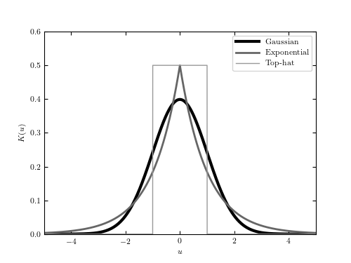
Figure 6.2
A comparison of the three kernels used for density estimation in figure 6.3: the Gaussian kernel (eq. 6.2), the top-hat kernel (eq. 6.3), and the exponential kernel (eq. 6.4).
# Author: Jake VanderPlas
# License: BSD
#   The figure produced by this code is published in the textbook
#   "Statistics, Data Mining, and Machine Learning in Astronomy" (2013)
#   For more information, see http://astroML.github.com
#   To report a bug or issue, use the following forum:
#    https://groups.google.com/forum/#!forum/astroml-general
import numpy as np
from matplotlib import pyplot as plt

#----------------------------------------------------------------------
# This function adjusts matplotlib settings for a uniform feel in the textbook.
# Note that with usetex=True, fonts are rendered with LaTeX.  This may
# result in an error if LaTeX is not installed on your system.  In that case,
# you can set usetex to False.
if "setup_text_plots" not in globals():
    from astroML.plotting import setup_text_plots
setup_text_plots(fontsize=8, usetex=True)

#------------------------------------------------------------
# Compute Kernels.
x = np.linspace(-5, 5, 10000)
dx = x[1] - x[0]

gauss = (1. / np.sqrt(2 * np.pi)) * np.exp(-0.5 * x ** 2)

exp = 0.5 * np.exp(-abs(x))

tophat = 0.5 * np.ones_like(x)
tophat[abs(x) > 1] = 0

#------------------------------------------------------------
# Plot the kernels
fig = plt.figure(figsize=(5, 3.75))
ax = fig.add_subplot(111)

ax.plot(x, gauss, '-', c='black', lw=3, label='Gaussian')
ax.plot(x, exp, '-', c='#666666', lw=2, label='Exponential')
ax.plot(x, tophat, '-', c='#999999', lw=1, label='Top-hat')

ax.legend(loc=1)

ax.set_xlabel('$u$')
ax.set_ylabel('$K(u)$')

ax.set_xlim(-5, 5)
ax.set_ylim(0, 0.6001)
plt.show()