Great Wall Density

Figure 6.4

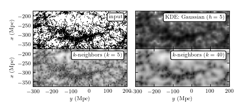
Density estimation for galaxies within the SDSS “Great Wall.” The upper-left panel shows points that are galaxies, projected by their spatial locations onto the equatorial plane (declination ~ 0 degrees). The remaining panels show estimates of the density of these points using kernel density estimation (with a Gaussian kernel with width 5Mpc), a K-nearest-neighbor estimator (eq. 6.15) optimized for a small-scale structure (with K = 5), and a K-nearest-neighbor estimator optimized for a large-scale structure (with K = 40).

Code output:

Python source code:

# Author: Jake VanderPlas
# License: BSD
#   The figure produced by this code is published in the textbook
#   "Statistics, Data Mining, and Machine Learning in Astronomy" (2013)
#   For more information, see http://astroML.github.com
#   To report a bug or issue, use the following forum:
#    https://groups.google.com/forum/#!forum/astroml-general

import numpy as np
from matplotlib import pyplot as plt
from matplotlib.colors import LogNorm

from sklearn.neighbors import KernelDensity
from astroML.datasets import fetch_great_wall
from astroML.density_estimation import KNeighborsDensity

#----------------------------------------------------------------------
# This function adjusts matplotlib settings for a uniform feel in the textbook.
# Note that with usetex=True, fonts are rendered with LaTeX.  This may
# result in an error if LaTeX is not installed on your system.  In that case,
# you can set usetex to False.
if "setup_text_plots" not in globals():
    from astroML.plotting import setup_text_plots
setup_text_plots(fontsize=8, usetex=True)

#------------------------------------------------------------
# Fetch the great wall data
X = fetch_great_wall()

#------------------------------------------------------------
# Create  the grid on which to evaluate the results
Nx = 50
Ny = 125
xmin, xmax = (-375, -175)
ymin, ymax = (-300, 200)

#------------------------------------------------------------
# Evaluate for several models
Xgrid = np.vstack(map(np.ravel, np.meshgrid(np.linspace(xmin, xmax, Nx),
                                            np.linspace(ymin, ymax, Ny)))).T

kde = KernelDensity(kernel='gaussian', bandwidth=5)
log_pdf_kde = kde.fit(X).score_samples(Xgrid).reshape((Ny, Nx))
dens_KDE = np.exp(log_pdf_kde)

knn5 = KNeighborsDensity('bayesian', 5)
dens_k5 = knn5.fit(X).eval(Xgrid).reshape((Ny, Nx))

knn40 = KNeighborsDensity('bayesian', 40)
dens_k40 = knn40.fit(X).eval(Xgrid).reshape((Ny, Nx))

#------------------------------------------------------------
# Plot the results
fig = plt.figure(figsize=(5, 2.2))
fig.subplots_adjust(left=0.12, right=0.95, bottom=0.2, top=0.9,
                    hspace=0.01, wspace=0.01)

# First plot: scatter the points
ax1 = plt.subplot(221, aspect='equal')
ax1.scatter(X[:, 1], X[:, 0], s=1, lw=0, c='k')
ax1.text(0.95, 0.9, "input", ha='right', va='top',
         transform=ax1.transAxes,
         bbox=dict(boxstyle='round', ec='k', fc='w'))

# Second plot: KDE
ax2 = plt.subplot(222, aspect='equal')
ax2.imshow(dens_KDE.T, origin='lower', norm=LogNorm(),
           extent=(ymin, ymax, xmin, xmax), cmap=plt.cm.binary)
ax2.text(0.95, 0.9, "KDE: Gaussian $(h=5)$", ha='right', va='top',
         transform=ax2.transAxes,
         bbox=dict(boxstyle='round', ec='k', fc='w'))

# Third plot: KNN, k=5
ax3 = plt.subplot(223, aspect='equal')
ax3.imshow(dens_k5.T, origin='lower', norm=LogNorm(),
           extent=(ymin, ymax, xmin, xmax), cmap=plt.cm.binary)
ax3.text(0.95, 0.9, "$k$-neighbors $(k=5)$", ha='right', va='top',
         transform=ax3.transAxes,
         bbox=dict(boxstyle='round', ec='k', fc='w'))

# Fourth plot: KNN, k=40
ax4 = plt.subplot(224, aspect='equal')
ax4.imshow(dens_k40.T, origin='lower', norm=LogNorm(),
           extent=(ymin, ymax, xmin, xmax), cmap=plt.cm.binary)
ax4.text(0.95, 0.9, "$k$-neighbors $(k=40)$", ha='right', va='top',
         transform=ax4.transAxes,
         bbox=dict(boxstyle='round', ec='k', fc='w'))

for ax in [ax1, ax2, ax3, ax4]:
    ax.set_xlim(ymin, ymax - 0.01)
    ax.set_ylim(xmin, xmax)

for ax in [ax1, ax2]:
    ax.xaxis.set_major_formatter(plt.NullFormatter())

for ax in [ax3, ax4]:
    ax.set_xlabel('$y$ (Mpc)')

for ax in [ax2, ax4]:
    ax.yaxis.set_major_formatter(plt.NullFormatter())

for ax in [ax1, ax3]:
    ax.set_ylabel('$x$ (Mpc)')

plt.show()

[download source: fig_great_wall.py]